June 2024, Week 5: June 24th - June 30th
June 24 -> 995. Minimum Number of K Consecutive Bit Flips
You are given a binary array nums and an integer k.
A k-bit flip is choosing a subarray of length k from nums and simultaneously changing every 0 in the subarray to 1, and every 1 in the subarray to 0.
Return the minimum number of k-bit flips required so that there is no 0 in the array. If it is not possible, return -1.
A subarray is a contiguous part of an array.
Example 1:
Input: nums = [0,1,0], k = 1
Output: 2
Explanation: Flip nums[0], then flip nums[2].
Example 2:
Input: nums = [1,1,0], k = 2
Output:-1
Explanation: No matter how we flip subarrays of size 2, we cannot make the array become [1,1,1].
Example 3:
Input: nums = [0,0,0,1,0,1,1,0], k = 3
Output: 3
Explanation:
Flip nums[0],nums[1],nums[2]: nums becomes [1,1,1,1,0,1,1,0]
Flip nums[4],nums[5],nums[6]: nums becomes [1,1,1,1,1,0,0,0]
Flip nums[5],nums[6],nums[7]: nums becomes [1,1,1,1,1,1,1,1]
Constraints:
1 <= nums.length <= 10^51 <= k <= nums.length
Approach 1: Sliding Window with Deque
Understanding the Core Idea
The central concept of this solution is to leverage a sliding window approach with a deque to efficiently track k-bit flips across the array. This method allows for optimized handling of overlapping flips without modifying the original array.
Sliding Window: A window of size
kis used to manage the effect of flips on each element.Deque for Flip Tracking: A deque efficiently tracks whether a flip occurred at each position within the current window.
Current Flipped State: This variable represents the cumulative effect of all flips on the current element.
Virtual Flips: Instead of actually modifying the array, the algorithm virtually flips elements by tracking the flip state.
Code Walkthrough
Initialization and Edge Case Handling:
if k == 1: return nums.count(0) flip_window_deque = deque() current_flipped_state = 0 total_flips = 0The function starts with an optimization for
k=1, simply counting the zeros. It then initializes the deque, the current flipped state, and the total flip count.Main Loop - Iterating Through the Array:
for index, num in enumerate(nums):This loop processes each element of the array, deciding whether to flip at each position.
Managing the Sliding Window:
if index >= k: current_flipped_state ^= flip_window_deque.popleft()When the window size exceeds
k, the effect of the oldest flip is removed using XOR operation.Flip Decision and Execution:
if current_flipped_state == num: if index + k > len(nums): return -1 flip_window_deque.append(1) current_flipped_state ^= 1 total_flips += 1 else: flip_window_deque.append(0)If the current state matches the original value, a flip is needed. The function checks if there's enough space for a flip, updates the deque and state, and increments the flip count. If no flip is needed, it appends 0 to the deque.
Result Calculation/Return:
return total_flipsAfter processing all elements, the function returns the total number of flips performed.
Complexity Analysis
Time Complexity:
, where is the length of the input array nums. This is because the algorithm processes each element of the array exactly once, performing constant-time operations for each element.
Space Complexity:
, where is the flip window size. This is due to the deque storing at most elements to track the sliding window of flips. The space used is independent of the input array size , making it more efficient for large arrays with smaller values.
Example
Input:
Step-by-Step Walkthrough:
Initialization:
flip_window_dequeis initialized as an empty deque:deque([])current_flipped_stateis set to 0total_flipsis set to 0
Main Loop (Iterating through
nums):Iteration 1 (index 0, num = 0):
current_flipped_state(0) ==num(0), so a flip is neededAdd 1 to
flip_window_deque:deque([1])Update
current_flipped_stateto 1Increment
total_flipsto 1
Iteration 2 (index 1, num = 0):
current_flipped_state(1) !=num(0), no flip neededAdd 0 to
flip_window_deque:deque([1, 0])
Iteration 3 (index 2, num = 0):
current_flipped_state(1) !=num(0), no flip neededAdd 0 to
flip_window_deque:deque([1, 0, 0])
Iteration 4 (index 3, num = 1):
Window size reached (
index >= k), remove oldest flip:deque([0, 0])Update
current_flipped_stateto 0current_flipped_state(0) !=num(1), no flip neededAdd 0 to
flip_window_deque:deque([0, 0, 0])
Iteration 5 (index 4, num = 0):
Remove oldest flip:
deque([0, 0])current_flipped_state(0) ==num(0), so a flip is neededAdd 1 to
flip_window_deque:deque([0, 0, 1])Update
current_flipped_stateto 1Increment
total_flipsto 2
Iteration 6 (index 5, num = 1):
Remove oldest flip:
deque([0, 1])current_flipped_state(1) ==num(1), so a flip is neededAdd 1 to
flip_window_deque:deque([0, 1, 1])Update
current_flipped_stateto 0Increment
total_flipsto 3
Iteration 7 (index 6, num = 1):
Remove oldest flip:
deque([1, 1])current_flipped_state(0) !=num(1), no flip neededAdd 0 to
flip_window_deque:deque([1, 1, 0])
Iteration 8 (index 7, num = 0):
Remove oldest flip:
deque([1, 0])Update
current_flipped_stateto 1current_flipped_state(1) !=num(0), no flip neededAdd 0 to
flip_window_deque:deque([1, 0, 0])
Loop Termination:
The loop ends after processing all elements in
numsFinal state:
total_flips= 3,current_flipped_state= 1,flip_window_deque=deque([1, 0, 0])
Visual Aid:
Iteration Summary Table:
Index
Element
Flipped State
Total Flips
Flip Window
0
0
1
1
[1]
1
0
1
1
[1, 0]
2
0
1
1
[1, 0, 0]
3
1
0
1
[0, 0, 0]
4
0
1
2
[0, 0, 1]
5
1
0
3
[0, 1, 1]
6
1
0
3
[1, 1, 0]
7
0
1
3
[1, 0, 0]
Result Calculation/Final Steps:
The algorithm arrives at the final result by counting the total number of flips performed
The final result is the value of
total_flips, which is 3
Approach 2: In-place Tracking with Active Flips
Understanding the Core Idea
The central concept of this solution is to use an in-place marking technique with clever bit manipulation to efficiently track k-bit flips across the array. This method combines the space efficiency of in-place modifications with an optimized approach to handling overlapping flips.
In-place Marking: The algorithm uses the value 2 to mark the start of a flip in the original array, enabling implicit storage of flip information without additional data structures.
Active Flips Tracking: An
active_flipsvariable keeps count of the number of active flips affecting the current element, allowing for quick flip decisions.Parity-based Flip Detection: The algorithm uses the parity of
active_flipsto determine whether the current element needs to be flipped.Virtual Flips: Instead of actually performing k-bit flips, the algorithm simulates their effect by tracking flip starts and active flip count.
Code Walkthrough
Initialization and Edge Case Handling:
if k == 1: return nums.count(0) n = len(nums) active_flips = 0 total_flips = 0The function starts with an optimization for
k=1, simply counting the zeros. It then initializes the length of the array, active flips count, and total flips count.Main Loop - Linear Scan:
for index in range(n):This loop processes each element of the array, making flip decisions based on the current state and previous flips.
Managing Active Flips:
if index >= k and nums[index - k] == 2: active_flips -= 1Flip Decision and Execution:
if (active_flips % 2) == nums[index]: if index + k > n: return -1 nums[index] = 2 active_flips += 1 total_flips += 1If the parity of active flips matches the current element's value, a flip is needed. The function checks if there's enough space for a flip, marks the flip start with 2, and updates the active and total flip counts.
Result Calculation/Return:
return total_flipsAfter processing all elements, the function returns the total number of flips performed.
Complexity Analysis
Time Complexity:
, where n is the length of the input array nums. This is because the algorithm processes each element of the array exactly once in the main loop, performing constant-time operations for each element.
Space Complexity:
, as the algorithm uses only a constant amount of extra space regardless of the input size. It cleverly uses the input array itself to store flip information by marking flip starts with the value 2, avoiding the need for additional data structures that grow with the input size.
Example
Input:
Step-by-Step Walkthrough:
Initialization:
nis set to 8 (length ofnums)active_flipsis set to 0total_flipsis set to 0
Main Loop (Iterating through
nums):Iteration 1 (index 0, num = 0):
No flip ending (index < k)
(active_flips % 2)(0) ==nums[0](0), so a flip is neededMark flip start:
nums[0] = 2Increment
active_flipsto 1Increment
total_flipsto 1
Iteration 2 (index 1, num = 0):
No flip ending (index < k)
(active_flips % 2)(1) !=nums[1](0), no flip needed
Iteration 3 (index 2, num = 0):
No flip ending (index < k)
(active_flips % 2)(1) !=nums[2](0), no flip needed
Iteration 4 (index 3, num = 1):
Flip ending:
nums[index - k](nums[0]) == 2Decrement
active_flipsto 0(active_flips % 2)(0) !=nums[3](1), no flip needed
Iteration 5 (index 4, num = 0):
No flip ending (
nums[1]!= 2)(active_flips % 2)(0) ==nums[4](0), so a flip is neededMark flip start:
nums[4] = 2Increment
active_flipsto 1Increment
total_flipsto 2
Iteration 6 (index 5, num = 1):
No flip ending (
nums[2]!= 2)(active_flips % 2)(1) ==nums[5](1), so a flip is neededMark flip start:
nums[5] = 2Increment
active_flipsto 2Increment
total_flipsto 3
Iteration 7 (index 6, num = 1):
No flip ending (
nums[3]!= 2)(active_flips % 2)(0) !=nums[6](1), no flip needed
Iteration 8 (index 7, num = 0):
Flip ending:
nums[index - k](nums[4]) == 2Decrement
active_flipsto 1(active_flips % 2)(1) !=nums[7](0), no flip needed
Loop Termination:
The loop ends after processing all elements in
numsFinal state:
total_flips= 3,active_flips= 1
Visual Aid:
Iteration Summary Table:
Index
Element Value
Active Flips
Total Flips
0
2
1
1
1
0
1
1
2
0
1
1
3
1
0
1
4
2
1
2
5
2
2
3
6
1
2
3
7
0
1
3
Result Calculation/Final Steps:
The algorithm arrives at the final result by counting the total number of flips performed
The final result is the value of
total_flips, which is 3
June 25 -> 1038. Binary Search Tree to Greater Sum Tree
Given the root of a Binary Search Tree (BST), convert it to a Greater Tree such that every key of the original BST is changed to the original key plus the sum of all keys greater than the original key in BST.
As a reminder, a binary search tree is a tree that satisfies these constraints:
The left subtree of a node contains only nodes with keys less than the node's key.
The right subtree of a node contains only nodes with keys greater than the node's key.
Both the left and right subtrees must also be binary search trees.
Example 1:
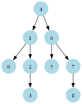
Input: root = [4,1,6,0,2,5,7,null,null,null,3,null,null,null,8]
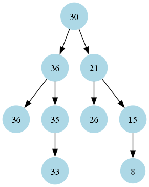
Output: [30,36,21,36,35,26,15,null,null,null,33,null,null,null,8]
Example 2:

Input: root = [0,null,1]
Output: [1,null,1]

Constraints:
The number of nodes in the tree is in the range
[1, 100].0 <= Node.val <= 100All the values in the tree are unique.
Approach 1: Recursive Reverse In-order Traversal
Understanding the Core Idea
The central concept of this solution is to leverage the properties of a Binary Search Tree (BST) to efficiently convert it into a Greater Sum Tree (GST). The solution uses a reverse in-order traversal (right-root-left) to accumulate the sum of greater values for each node.
BST Property Exploitation: In a BST, all nodes in the right subtree have greater values than the current node, and all nodes in the left subtree have smaller values.
Reverse In-order Traversal: By traversing the tree in a right-root-left order, we process larger values first, allowing us to accumulate the sum of greater values for each node.
Cumulative Sum Propagation: As we traverse, we maintain a running sum of all greater values, updating each node's value with this sum plus its original value.
Code Walkthrough
Initialization:
cumulative_sum = 0A variable
cumulative_sumis initialized to 0. This will be used to keep track of the running sum of greater values as we traverse the tree.Helper Function Definition:
def update_node_values(node: TreeNode) -> None: nonlocal cumulative_sumAn inner function
update_node_valuesis defined to perform the recursive traversal and node value updates. It uses thenonlocalkeyword to access and modify thecumulative_sumvariable from the outer scope.Right Subtree Traversal:
if node.right: update_node_values(node.right)The function first recursively processes the right subtree, ensuring that all greater values are processed before the current node.
Node Value Update:
cumulative_sum += node.val node.val = cumulative_sumAfter processing the right subtree, the current node's original value is added to
cumulative_sum, and then the node's value is updated to be this new sum.Left Subtree Traversal:
if node.left: update_node_values(node.left)Finally, the function recursively processes the left subtree, which will use the updated
cumulative_sumthat now includes the current node's original value.Traversal Initiation and Return:
update_node_values(root) return rootThe traversal is started by calling
update_node_valueson the root node. After the traversal is complete, the modified root is returned.
Complexity Analysis
Time Complexity:
, where is the number of nodes in the tree. This is because each node in the tree is visited exactly once during the traversal.
Space Complexity:
, where is the height of the tree. This space is used by the recursive call stack. In the worst case of an unbalanced tree (skewed tree), this could be , but for a balanced BST, it would be .
The space complexity is determined by the maximum depth of the recursive call stack, which corresponds to the height of the tree. Each recursive call adds a frame to the call stack, and the maximum number of simultaneous frames is equal to the height of the tree.
Example
Input:
A visual representation of the input BST:

Step-by-Step Walkthrough:
Initialization:
Set
cumulative_sum = 0Call
update_node_values(root)with the root node (4)
Main Loop (Reverse In-order Traversal):
Iteration 1 (Node 4):
Move to right child (6)
Iteration 2 (Node 6):
Move to right child (7)
Iteration 3 (Node 7):
Move to right child (8)
Iteration 4 (Node 8):
No right child, process node
Update
cumulative_sum: 0 + 8 = 8Set node value to 8
No left child, return to parent (7)
Iteration 5 (Node 7):
Update
cumulative_sum: 8 + 7 = 15Set node value to 15
No left child, return to parent (6)
Iteration 6 (Node 6):
Update
cumulative_sum: 15 + 6 = 21Set node value to 21
Move to left child (5)
Iteration 7 (Node 5):
No right child, process node
Update
cumulative_sum: 21 + 5 = 26Set node value to 26
No left child, return to parent (6), then to grandparent (4)
Iteration 8 (Node 4):
Update
cumulative_sum: 26 + 4 = 30Set node value to 30
Move to left child (1)
Iteration 9 (Node 1):
Move to right child (2)
Iteration 10 (Node 2):
Move to right child (3)
Iteration 11 (Node 3):
No right child, process node
Update
cumulative_sum: 30 + 3 = 33Set node value to 33
No left child, return to parent (2)
Iteration 12 (Node 2):
Update
cumulative_sum: 33 + 2 = 35Set node value to 35
No left child, return to parent (1)
Iteration 13 (Node 1):
Update
cumulative_sum: 35 + 1 = 36Set node value to 36
Move to left child (0)
Iteration 14 (Node 0):
No right child, process node
Update
cumulative_sum: 36 + 0 = 36Set node value to 36
No left child, return to parent (1), then to grandparent (4)
Loop Termination:
The traversal is complete when we return to the root node (4) and there are no more nodes to visit
Final
cumulative_sumis 36
Visual Aid:
Iteration Summary Table:
Original Value
Added to Sum
New Value (Cumulative Sum)
8
0
8
7
8
15
6
15
21
5
21
26
4
26
30
3
30
33
2
33
35
1
35
36
0
36
36
Result Calculation/Final Steps:
The algorithm has modified the BST in-place
Each node's value now represents the sum of its original value and all greater values in the original BST
The root node (originally 4) now has the value 30, which is the sum of 4 and all greater values (5, 6, 7, 8)
The resulting Greater Sum Tree maintains the BST structure but with updated node values
The final Greater Sum Tree looks like this:

Approach 2: Iterative Reverse In-order Traversal with Stack
Understanding the Core Idea
The central concept of this solution is to convert a Binary Search Tree (BST) to a Greater Sum Tree (GST) using an iterative approach with a stack. This method simulates the reverse in-order traversal (right-root-left) without using recursion.
Iterative Traversal: Instead of recursion, the solution uses a stack to keep track of nodes to be processed, allowing for an iterative implementation.
Right-First Approach: By pushing all right nodes onto the stack first, the algorithm ensures that larger values are processed before smaller ones.
Cumulative Sum Propagation: As in the recursive version, a running sum is maintained and used to update node values.
Code Walkthrough
Helper Function Definition:
def push_right_nodes(node: TreeNode) -> None: while node: stack.append(node) node = node.rightThis helper function pushes all right child nodes of a given node onto the stack. It's crucial for maintaining the right-root-left traversal order.
Initialization:
stack = [] current_node = root cumulative_sum = 0A stack is initialized to store nodes,
current_nodeis set to the root, andcumulative_sumis initialized to 0 to keep track of the running sum.Initial Stack Population:
push_right_nodes(current_node)The stack is initially populated with the root and all its right descendants.
Main Traversal Loop:
while stack:The main loop continues as long as there are nodes in the stack to process.
Node Processing:
current_node = stack.pop() cumulative_sum += current_node.val current_node.val = cumulative_sumFor each node, we pop it from the stack, add its value to the cumulative sum, and then update its value with this new sum.
Left Subtree Handling:
push_right_nodes(current_node.left)After processing a node, we push all right descendants of its left child onto the stack. This ensures that we process the left subtree after the current node, maintaining the reverse in-order traversal.
Result Return:
return rootAfter processing all nodes, the modified root is returned.
Complexity Analysis
Time Complexity:
, where is the number of nodes in the tree. Each node is visited exactly once during the traversal. Although we have a nested loop (the whileloop inpush_right_nodesinside the mainwhileloop), each node is still pushed and popped from the stack exactly once.
Space Complexity:
, where h is the height of the tree. The stack uses this space to store nodes during traversal. In the worst case of an unbalanced tree (skewed tree), this could be , but for a balanced BST, it would be .
The space complexity is determined by the maximum number of nodes that can be on the stack at any given time. This corresponds to the height of the tree because, at most, we will have a path from the root to a leaf on the stack.
Example
Input:
A visual representation of the input BST:

Step-by-Step Walkthrough:
Initialization:
Initialize an empty
stack = []Set
current_node = root(4)Set
cumulative_sum = 0
Initial Stack Population:
Call
push_right_nodes(current_node)Push 4 onto the stack
Move to right child: 6
Push 6 onto the stack
Move to right child: 7
Push 7 onto the stack
Move to right child: 8
Push 8 onto the stack
No more right children
Stack after pushing: [4, 6, 7, 8]
Main Traversal Loop:
Iteration 1 (Node 8):
Pop 8 from the stack
Update
cumulative_sum: 0 + 8 = 8Set node value to 8
No left child to process
Iteration 2 (Node 7):
Pop 7 from the stack
Update
cumulative_sum: 8 + 7 = 15Set node value to 15
No left child to process
Iteration 3 (Node 6):
Pop 6 from the stack
Update
cumulative_sum: 15 + 6 = 21Set node value to 21
Process left child (5):
Push 5 onto the stack
Stack after pushing: [4, 5]
Iteration 4 (Node 5):
Pop 5 from the stack
Update
cumulative_sum: 21 + 5 = 26Set node value to 26
No left child to process
Iteration 5 (Node 4):
Pop 4 from the stack
Update
cumulative_sum: 26 + 4 = 30Set node value to 30
Process left child (1):
Push 1 onto the stack
Move to right child: 2
Push 2 onto the stack
Move to right child: 3
Push 3 onto the stack
Stack after pushing: [1, 2, 3]
Iteration 6 (Node 3):
Pop 3 from the stack
Update
cumulative_sum: 30 + 3 = 33Set node value to 33
No left child to process
Iteration 7 (Node 2):
Pop 2 from the stack
Update
cumulative_sum: 33 + 2 = 35Set node value to 35
No left child to process
Iteration 8 (Node 1):
Pop 1 from the stack
Update
cumulative_sum: 35 + 1 = 36Set node value to 36
Process left child (0):
Push 0 onto the stack
Stack after pushing: [0]
Iteration 9 (Node 0):
Pop 0 from the stack
Update
cumulative_sum: 36 + 0 = 36Set node value to 36
No left child to process
Visual Aid:
Iteration Summary Table:
Original Value
Added to Sum
New Value (Cumulative Sum)
8
0
8
7
8
15
6
15
21
5
21
26
4
26
30
3
30
33
2
33
35
1
35
36
0
36
36
Result Calculation/Final Steps:
The algorithm has modified the BST in-place
Each node's value now represents the sum of its original value and all greater values in the original BST
The root node (originally 4) now has the value 30, which is the sum of 4 and all greater values (5, 6, 7, 8)
The resulting Greater Sum Tree maintains the BST structure but with updated node values
The final Greater Sum Tree looks like this:

This iterative approach using a stack achieves the same result as the recursive method, converting the BST to a Greater Sum Tree by updating each node's value to be the sum of its original value and all greater values in the tree.
Approach 3: Morris Traversal
Understanding the Core Idea
The central concept of this solution is to convert a Binary Search Tree (BST) to a Greater Sum Tree (GST) using the Morris Traversal algorithm. This method performs a reverse in-order traversal (right-root-left) without using recursion or an explicit stack, achieving
Morris Traversal: This technique creates temporary links in the tree to facilitate navigation without additional data structures.
Threaded Binary Tree: The algorithm temporarily modifies the tree structure, creating links from successor nodes to their predecessors.
Constant Space: By using these temporary links, the traversal is performed using only a constant amount of extra space, regardless of tree size.
Code Walkthrough
Helper Function Definition:
def find_successor(current_node: TreeNode) -> TreeNode: successor = current_node.right while successor.left and successor.left is not current_node: successor = successor.left return successorThis function finds the inorder successor (leftmost node of the right subtree) of the current node in the context of reverse inorder traversal.
Initialization:
cumulative_sum = 0 current_node = rootcumulative_sumis initialized to keep track of the running sum, andcurrent_nodeis set to the root to begin traversal.Main Traversal Loop:
while current_node:The main loop continues as long as there's a current node to process.
No Right Child Case:
if not current_node.right: cumulative_sum += current_node.val current_node.val = cumulative_sum current_node = current_node.leftIf there's no right child, we process the current node and move to the left.
Right Child Exists Case:
else: successor = find_successor(current_node)If a right child exists, we find the successor node.
First Visit to Successor:
if not successor.left: successor.left = current_node current_node = current_node.rightOn the first visit, we create a temporary link from the successor to the current node and move right.
Second Visit to Successor:
else: successor.left = None cumulative_sum += current_node.val current_node.val = cumulative_sum current_node = current_node.leftOn the second visit, we remove the temporary link, process the current node, and move left.
Result Return:
return rootAfter processing all nodes, the modified root is returned.
Complexity Analysis
Time Complexity:
, where is the number of nodes in the tree. Although each node may be visited up to three times (to create the link, to process the node, and to remove the link), this still results in linear time complexity. The total number of operations is proportional to the number of nodes.
Space Complexity:
, constant space. This is the key advantage of Morris Traversal. It uses only a constant amount of extra space, regardless of the tree size. The temporary modifications to the tree structure do not count towards space complexity as they are made within the existing tree nodes and are reverted during the traversal.
The constant space complexity is achieved by using the existing tree structure to simulate the traversal stack, avoiding the need for additional data structures that grow with the size of the input.
Example
Input:
A visual representation of the input BST:

Step-by-Step Walkthrough:
Initialization:
Set
cumulative_sum = 0Set
current_node = root(4)
Main Traversal Loop:
Processing Node 4:
Find successor: 5 (leftmost node of right subtree)
Create temporary link: 5.left = 4
Move to right child: 6
Processing Node 6:
Find successor: 7
Create temporary link: 7.left = 6
Move to right child: 7
Processing Node 7:
Find successor: 8
Create temporary link: 8.left = 7
Move to right child: 8
Processing Node 8:
No right child
Update node: 8 + 0 = 8
Move to left child: 7
Processing Node 7 (second visit):
Remove temporary link: 8.left = None
Update node: 7 + 8 = 15
Move to left child: 6
Processing Node 6 (second visit):
Remove temporary link: 15.left = None
Update node: 6 + 15 = 21
Move to left child: 5
Processing Node 5:
No right child
Update node: 5 + 21 = 26
Move to left child: 4
Processing Node 4 (second visit):
Remove temporary link: 26.left = None
Update node: 4 + 26 = 30
Move to left child: 1
Processing Node 1:
Find successor: 2
Create temporary link: 2.left = 1
Move to right child: 2
Processing Node 2:
Find successor: 3
Create temporary link: 3.left = 2
Move to right child: 3
Processing Node 3:
No right child
Update node: 3 + 30 = 33
Move to left child: 2
Processing Node 2 (second visit):
Remove the temporary link: 33.left = None
Update node: 2 + 33 = 35
Move to left child: 1
Processing Node 1 (second visit):
Remove the temporary link: 35.left = None
Update node: 1 + 35 = 36
Move to left child: 0
Processing Node 0:
No right child
Update node: 0 + 36 = 36
Move to left child: None (Traversal complete)
Visual Aid:
Iteration Summary Table:
Original Value
Added to Sum
New Value (Cumulative Sum)
8
0
8
7
8
15
6
15
21
5
21
26
4
26
30
3
30
33
2
33
35
1
35
36
0
36
36
Result Calculation/Final Steps:
The algorithm has modified the BST in-place
Each node's value now represents the sum of its original value and all greater values in the original BST
The root node (originally 4) now has the value 30, which is the sum of 4 and all greater values (5, 6, 7, 8)
The resulting Greater Sum Tree maintains the BST structure but with updated node values
All temporary links created during the traversal have been removed, restoring the original tree structure
The final Greater Sum Tree looks like this:

This Morris Traversal approach achieves the same result as the recursive and stack-based methods, converting the BST to a Greater Sum Tree. It does so without using additional data structures (like a stack) or recursive calls, maintaining
June 26 -> 1382. Balance a Binary Search Tree
Given the root of a binary search tree, return a balanced binary search tree with the same node values. If there is more than one answer, return any of them.
A binary search tree is balanced if the depth of the two subtrees of every node never differs by more than 1.
Example 1:
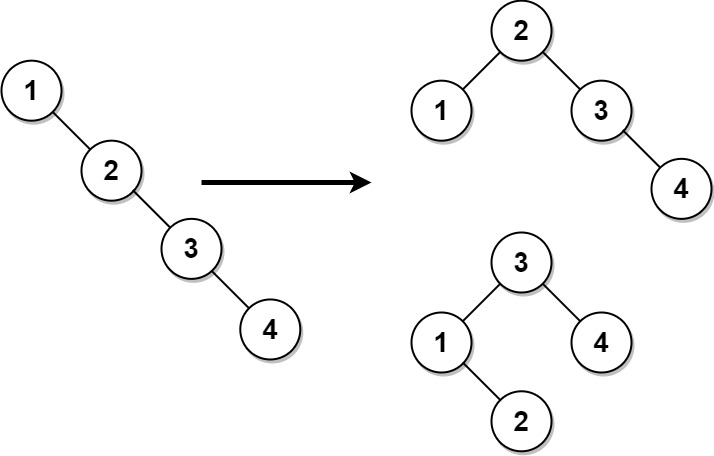
Input: root = [1,null,2,null,3,null,4,null,null]
Output: [2,1,3,null,null,null,4]
Explanation: This is not the only correct answer, [3,1,4,null,2] is also correct.
Example 2:
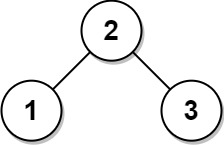
Input: root = [2,1,3]
Output: [2,1,3]
Constraints:
The number of nodes in the tree is in the range
[1, 10^4].1 <= Node.val <= 10^5
Approach 1: In-Order Traversal and Recursive Reconstruction
Understanding the Core Idea
The central concept of this solution is to leverage the properties of Binary Search Trees (BSTs) and in-order traversal to create a balanced BST. This approach consists of two main steps:
In-Order Traversal: Perform an in-order traversal of the original BST to get a sorted list of nodes.
Recursive Reconstruction: Use the sorted list to recursively construct a new balanced BST.
BST Property Exploitation: In-order traversal of a BST yields nodes in ascending order, which is crucial for the balancing step.
Divide and Conquer: The reconstruction phase uses a divide-and-conquer approach, selecting the median element as the root at each step to ensure balance.
Code Walkthrough
Initialization and Helper Function Definitions:
def balanceBST1(root: TreeNode) -> TreeNode: inorder_nodes = [] def inorder_traverse(root: TreeNode) -> None: # ... (implementation details in step 2) def build_balanced_bst(start_index: int, end_index: int) -> TreeNode | None: # ... (implementation details in step 3)The main function
balanceBST1is defined, along with an empty listinorder_nodesto store the sorted nodes. Two helper functions,inorder_traverseandbuild_balanced_bstare also defined within the main function's scope.In-Order Traversal:
def inorder_traverse(root: TreeNode) -> None: if not root: return inorder_traverse(root.left) inorder_nodes.append(root) inorder_traverse(root.right)This helper function performs an in-order traversal of the original BST. It recursively visits the left subtree, appends the current node to
inorder_nodes, and then visits the right subtree. This results in a list of nodes sorted in ascending order.Balanced BST Construction:
def build_balanced_bst(start_index: int, end_index: int) -> TreeNode | None: if start_index > end_index: return None mid_index = start_index + (end_index - start_index) // 2 node = inorder_nodes[mid_index] node.left = build_balanced_bst(start_index, mid_index - 1) node.right = build_balanced_bst(mid_index + 1, end_index) return nodeThis helper function recursively constructs a balanced BST from the sorted list of nodes. It selects the middle element as the root, recursively builds the left subtree from nodes before the middle, and the right subtree from nodes after the middle.
Execution and Return:
inorder_traverse(root) return build_balanced_bst(0, len(inorder_nodes) - 1)Finally, the main function executes the in-order traversal on the input tree and then calls
build_balanced_bstto construct and return the balanced BST.
Complexity Analysis
Time Complexity:
, where is the number of nodes in the tree. This is because: The in-order traversal visits each node once:
The balanced BST construction processes each node once:
The total time is the sum of these operations:
Space Complexity:
, where is the number of nodes in the tree. This is because: The
inorder_nodeslist stores all n nodes:The recursion stack in both traversal and construction can go up to
in the balanced case, but in the worst case (skewed tree) The total space is dominated by the largest of these:
Example
Input:
A visual representation of the input BST:

Step-by-Step Walkthrough:
Initialization:
An empty list
inorder_nodesis created to store the nodes in sorted order.
In-order Traversal:
Node 4:
The function starts at the root node with value 4.
It moves to the left child (node 3).
Node 3:
The function moves to the left child (node 2).
Node 2:
The function moves to the left child (node 1).
Node 1:
The function checks the left child, which is
None.Node 1 is appended to
inorder_nodes.inorder_nodes = [1]
The function checks the right child, which is
None.The function returns to node 2.
Back to Node 2:
Node 2 is appended to
inorder_nodes.inorder_nodes = [1, 2]
The function checks the right child, which is
None.The function returns to node 3.
Back to Node 3:
Node 3 is appended to
inorder_nodes.inorder_nodes = [1, 2, 3]
The function checks the right child, which is
None.The function returns to node 4.
Back to Node 4:
Node 4 is appended to
inorder_nodes.inorder_nodes = [1, 2, 3, 4]
The function checks the right child, which is
None.The in-order traversal is complete.
Building Balanced BST:
Initial Call:
start_index = 0,end_index = 3mid_index = 1Root node is set to
inorder_nodes[1](value 2)Left and right subtrees are recursively constructed.
Left subtree: from
start_indextomid_index - 1(0 to 0)Right subtree: from
mid_index + 1toend_index(2 to 3)
Left Subtree (0, 0):
start_index = 0,end_index = 0mid_index = 0Node with value 1 becomes the left child of 2
Its left and right children are set to
Nonebecause the index range will be invalid
Right Subtree (2, 3):
start_index = 2,end_index = 3mid_index = 2Node with value 3 becomes the right child of 2
Left and right subtrees are recursively constructed.
Left subtree: from
start_indextomid_index - 1(2 to 1) - Invalid rangeRight subtree: from
mid_index + 1toend_index(3 to 3)
Right Subtree of 3 (3, 3):
start_index = 3,end_index = 3mid_index = 3Node with value 4 becomes the right child of 3
Its left and right children are set to
Nonebecause the index range will be invalid
Result Calculation:
The function returns the root of the new balanced BST (node with value 2).
The depth of every node in the new tree differs by at most 1, satisfying the balance condition.
A visual representation of the output Balanced BST:

Approach 2: Day-Stout-Warren (DSW) Algorithm
Understanding the Core Idea
The central concept of this solution is to leverage the Day-Stout-Warren (DSW) algorithm to balance the Binary Search Tree (BST). This approach consists of three main steps:
Vine Creation: Convert the BST into a "vine" (a right-skewed tree).
Perfect Tree Size Calculation: Determines the number of nodes needed for a perfect binary tree. A perfect binary tree is a binary tree in which all levels are filled except possibly for the lowest level, which is filled from left to right.
Tree Balancing: Perform a series of left rotations to balance the tree.
In-Place Transformation: The DSW algorithm achieves balance through a series of tree rotations, without requiring extra space for node storage.
Guaranteed Balance: It ensures a balanced tree with a height of
. Space Efficiency: Unlike methods that require
auxiliary space, this approach uses only extra space.
Code Walkthrough
Helper Function Definitions:
def right_rotate(parent: TreeNode, node: TreeNode) -> None: left_child = node.left node.left = left_child.right left_child.right = node parent.right = left_childThe
right_rotatefunction performs a right rotation on the given node:It saves the left child of the node.
It sets the node's left child to be the right child of its former left child.
It makes the node the right child of its former left child.
It updates the parent to point to the new root of this subtree (the former left child).
def left_rotate(parent: TreeNode, node: TreeNode) -> None: right_child = node.right node.right = right_child.left right_child.left = node parent.right = right_childThe
left_rotatefunction performs a left rotation on the given node:It saves the right child of the node.
It sets the node's right child to be the left child of its former right child.
It makes the node the left child of its former right child.
It updates the parent to point to the new root of this subtree (the former right child).
def compress_vine(vine_root: TreeNode, rotations: int) -> None: current_node = vine_root for _ in range(rotations): child = current_node.right left_rotate(current_node, child) current_node = current_node.rightThe
compress_vinefunction performs a series of left rotations to balance part of the vine:It starts from the
vine_rootand performs the specified number ofrotations.For each rotation, it performs a left rotation on the current node's right child.
After each rotation, it moves to the new right child to continue the process.
Initialization:
dummy_root = TreeNode() dummy_root.right = root current_node = dummy_rootA dummy root is created to handle edge cases and simplify the vine creation process. The original root becomes the right child of this dummy node.
Vine Creation (Step 1):
while current_node.right: if current_node.right.left: right_rotate(current_node, current_node.right) else: current_node = current_node.rightThis loop converts the BST into a right-skewed tree (vine) by performing right rotations whenever a left child is encountered.
Node Counting and Perfect Tree Size Calculation (Step 2):
node_count = 0 current_node = dummy_root.right while current_node: node_count += 1 current_node = current_node.right perfect_tree_nodes = 2 ** math.floor(math.log2(node_count + 1)) - 1This section counts the total number of nodes and calculates the size of the largest perfect binary tree that can be formed with these nodes. The perfect tree size is determined by finding the largest power of 2 less than or equal to the node count. This is expressed as
. Tree Balancing (Step 3):
compress_vine(dummy_root, node_count - perfect_tree_nodes) remaining_nodes = perfect_tree_nodes while remaining_nodes > 1: remaining_nodes //= 2 compress_vine(dummy_root, remaining_nodes)The balancing process involves an initial compression to remove excess nodes, followed by a series of compressions that transform the vine into a balanced tree. Here we perform the initial compression and then iteratively reduce the number of remaining nodes by half, performing compressions at each step.
Result Return:
return dummy_root.rightThe function returns the right child of the dummy root, which is the root of the balanced BST.
Complexity Analysis
Time Complexity:
, where is the number of nodes in the tree. This is because: Vine creation visits each node at most once:
Node counting is a linear traversal:
Tree balancing performs a constant number of operations per node:
Despite multiple passes, each node is processed a constant number of times, resulting in linear time complexity.
Space Complexity:
, which is constant space. This is because: The algorithm uses only a fixed number of additional variables (e.g.,
dummy_root,current_node)All operations are performed in-place, without requiring additional data structures that grow with input size
The recursion depth (or iteration count) in helper functions is independent of the tree size
This space efficiency is a key advantage of the DSW algorithm, especially for large trees where
Example
Input:
A visual representation of the input BST:

Step-by-Step Walkthrough:
Initialization:
A dummy root is created and connected to the tree root.
The
current_nodeis set to the dummy root.
Step 1: Convert BST to vine (right-leaning linked list)
We start with
current_nodeas the dummy root.We continue this process while
current_node.rightexists.If
current_node.right.leftexists, we perform a right rotation.Otherwise, we move
current_nodetocurrent_node.right.Right Rotation 1:
current_nodeis dummy,current_node.rightis 4, andcurrent_node.right.leftis 3.We perform a right rotation:
Set
left_child = node.left(left_child = 3)Set
node.left = left_child.right(4.left = None)Set
left_child.right = node(3.right = 4)Set
parent.right = left_child(dummy.right = 3)
After rotation:
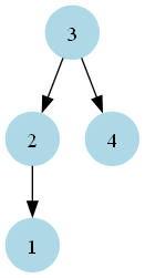
Right Rotation 2:
current_nodeis still dummy,current_node.rightis now 3, andcurrent_node.right.leftis 2.We perform another right rotation:
Set
left_child = node.left(left_child = 2)Set
node.left = left_child.right(3.left = None)Set
left_child.right = node(2.right = 3)Set
parent.right = left_child(dummy.right = 2)
After rotation:
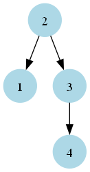
Right Rotation 3:
current_nodeis still dummy,current_node.rightis now 2, andcurrent_node.right.leftis 1.We perform the final right rotation:
Set
left_child = node.left(left_child = 1)Set
node.left = left_child.right(2.left = None)Set
left_child.right = node(1.right = 2)Set
parent.right = left_child(dummy.right = 1)
After rotation:

Vine creation complete:
The BST is now a right-leaning linked list (vine)
Vine nodes: [1, 2, 3, 4]
Step 2: Count nodes and calculate perfect tree size
We traverse the vine to count the nodes:
Start with
current_node = dummy_root.rightWhile
current_nodeexists, incrementnode_countand move tocurrent_node.right
Total node count: 4
Calculate perfect tree nodes:
Step 3: Balance the tree through a series of left rotations
We perform compressions to balance the tree.
Initial Compression (1 rotation):
Number of rotations = node_count - perfect_tree_nodes = 4 - 3 = 1
We perform 1 left rotation:
Set
right_child = node.right(right_child = 2)Set
node.right = right_child.left(1.right = None)Set
right_child.left = node(2.left = 1)Set
parent.right = right_child(dummy.right = 2)
After compression (Left rotation):

Remaining Compression (1 rotation):
We calculate remaining_nodes = perfect_tree_nodes = 3
While remaining_nodes > 1, we divide it by 2: 3 // 2 = 1
We perform one more left rotation:
Set
right_child = node.right(right_child = 3)Set
node.right = right_child.left(2.right = None)Set
right_child.left = node(3.left = 2)Set
parent.right = right_child(dummy.right = 3)
After compression (Left rotation):

Compression Summary:
Initial compressions: 1
Compression rounds: [1]
Final Balanced Tree:
The tree is now balanced, with a height difference of at most 1 between any two subtrees.

June 27 -> 1791. Find Center of Star Graph
There is an undirected star graph consisting of n nodes labeled from 1 to n. A star graph is a graph where there is one center node and exactly n - 1 edges that connect the center node with every other node.
You are given a 2D integer array edges where each edges[i] = [u_i, v_i] indicates that there is an edge between the nodes u_i and v_i. Return the center of the given star graph.
Example 1:
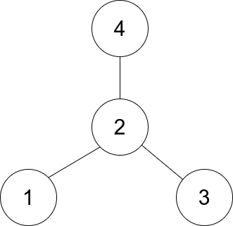
Input: edges = [[1,2],[2,3],[4,2]]
Output: 2
Explanation: As shown in the figure above, node 2 is connected to every other node, so 2 is the center.
Example 2:
Input: edges = [[1,2],[5,1],[1,3],[1,4]]
Output: 1
Constraints:
3 <= n <= 10^5edges.length == n - 1edges[i].length == 21 <= u_i, v_i <= nu_i != viThe given
edgesrepresent a valid star graph.
Approach 1: Two-Edge Comparison
Understanding the Core Idea
The central concept of this solution is to leverage the unique property of a star graph to efficiently identify the center node. In a star graph, the center node is connected to all other nodes, which means it appears on every edge.
Minimum Edge Requirement: We only need to examine two edges to find the center node.
Common Node Principle: The center node will be the only node that appears in both of these edges.
Code Walkthrough
Function Definition and Edge Selection:
def findCenter1(edges: List[List[int]]) -> int: reference_edge, comparison_edge = edges[0], edges[1]The function takes a list of edges as input. It immediately selects the first two edges from this list, assigning them to
reference_edgeandcomparison_edge. This selection is arbitrary but sufficient due to the star graph's properties.Center Node Identification:
return (reference_edge[0] if reference_edge[0] in comparison_edge else reference_edge[1])This single line performs the core logic of the function:
It checks if the first node of the
reference_edgeis present in thecomparison_edge.If true, this node must be the center (as it's in both edges) and is returned.
If false, the second node of the
reference_edgemust be the center (since one of the two must be the center, and we've eliminated the first).
Complexity Analysis
Time Complexity:
, where is the number of nodes in the graph. This is because the function performs a fixed number of operations regardless of the input size. It only accesses two edges and performs a single comparison.
Space Complexity:
. The function uses only a constant amount of extra space to store the two selected edges and perform the comparison, regardless of the input size.
Example
Input:
Step-by-Step Walkthrough:
Initialization:
The function receives the
edgeslist as input.reference_edgeis set to[1, 2](the first edge in the list).comparison_edgeis set to[5, 1](the second edge in the list).
Center Node Identification:
The function checks if the first node of
reference_edge(1) is incomparison_edge[5, 1].Condition:
1 in [5, 1]evaluates toTrue.Since the condition is true, the center node is identified as 1.
Visual Aids: A decision summary table is created:
Reference Edge
Comparison Edge
Condition
Center Node
[1, 2]
[5, 1]
1 in [5, 1]
1
Result Calculation/Final Steps:
The function determines that 1 is the center node.
This is correct because node 1 appears in all edges of the input, confirming it's connected to all other nodes.
June 28 -> 2285. Maximum Total Importance of Roads
You are given an integer n denoting the number of cities in a country. The cities are numbered from 0 to n - 1.
You are also given a 2D integer array roads where roads[i] = [a_i, b_i] denotes that there exists a bidirectional road connecting cities a_i and b_i.
You need to assign each city with an integer value from 1 to n, where each value can only be used once. The importance of a road is then defined as the sum of the values of the two cities it connects.
Return the maximum total importance of all roads possible after assigning the values optimally.
Example 1:
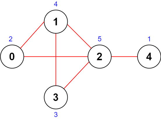
Input: n = 5, roads = [[0,1],[1,2],[2,3],[0,2],[1,3],[2,4]]
Output: 43
Explanation: The figure above shows the country and the assigned values of [2,4,5,3,1].
The road (0,1) has importance of 2 + 4 = 6.
The road (1,2) has importance of 4 + 5 = 9.
The road (2,3) has importance of 5 + 3 = 8.
The road (0,2) has importance of 2 + 5 = 7.
The road (1,3) has importance of 4 + 3 = 7.
The road (2,4) has importance of 5 + 1 = 6.
The total importance of all roads is 6 + 9 + 8 + 7 + 7 + 6 = 43.
It can be shown that we cannot get greater total importance than 43.
Example 2:
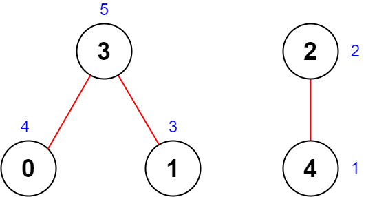
Input: n = 5, roads = [[0,3],[2,4],[1,3]]
Output: 20
Explanation: The figure above shows the country and the assigned values of [4,3,2,5,1].
The road (0,3) has importance of 4 + 5 = 9.
The road (2,4) has importance of 2 + 1 = 3.
The road (1,3) has importance of 3 + 5 = 8.
The total importance of all roads is 9 + 3 + 8 = 20.
It can be shown that we cannot get greater total importance than 20.
Constraints:
2 <= n <= 5 * 10^41 <= roads.length <= 5 * 10^4roads[i].length == 20 <= a_i, b_i <= n - 1a_i != b_iThere are no duplicate roads.
Approach 1: Greedy Assignment with Connection Count
Understanding the Core Idea
The central concept of this solution is to leverage a greedy approach to maximize the total importance of roads. The key insight is that assigning higher values to cities with more connections will result in the maximum total importance.
Connection Count: The solution starts by counting how many connections each city has.
Value Assignment: Cities are then assigned values from 1 to n based on their connection count, with more connected cities receiving higher values.
Greedy Strategy: This greedy strategy ensures that the cities contributing to more roads get higher values, thus maximizing the overall importance.
Code Walkthrough
Initialization and Connection Counting:
city_connections = [0] * n for city1, city2 in roads: city_connections[city1] += 1 city_connections[city2] += 1This step initializes a list
city_connectionsto keep track of how many roads are connected to each city. It then iterates through theroadslist, incrementing the count for both cities connected by each road.Initialization of Result Variables:
total_importance = 0 city_value = 1total_importancewill store the final result, whilecity_valueis used to assign increasing values to cities.Sorting and Importance Calculation:
for connections in sorted(city_connections): total_importance += city_value * connections city_value += 1This is the core of the algorithm. It sorts the
city_connectionslist, effectively ordering cities from least to most connected. Then, it iterates through this sorted list, calculating the contribution to the total importance for each city and incrementing thecity_valuefor the next iteration.Result Return:
return total_importanceThe final calculated
total_importanceis returned as the result.
Complexity Analysis
Time Complexity:
, where is the number of cities and is the number of roads. Counting connections:
Sorting the connection counts:
Final calculation loop:
The overall complexity is dominated by the sorting step, hence
.
Space Complexity:
, where is the number of cities. The
city_connectionslist usesspace. The sorting operation in Python (Timsort) uses
space in the worst case. All other variables use constant space.
Example
Input:
Step-by-Step Walkthrough:
Initialization:
We start with
n = 5cities and a list ofroadsconnecting them.Initialize
city_connections = [0, 0, 0, 0, 0], a list to count connections for each city.
Counting Connections:
Iterate through each road in
roads:Road 1: 0 <-> 1 → Update:
city_connections = [1, 1, 0, 0, 0]Road 2: 1 <-> 2 → Update:
city_connections = [1, 2, 1, 0, 0]Road 3: 2 <-> 3 → Update:
city_connections = [1, 2, 2, 1, 0]Road 4: 0 <-> 2 → Update:
city_connections = [2, 2, 3, 1, 0]Road 5: 1 <-> 3 → Update:
city_connections = [2, 3, 3, 2, 0]Road 6: 2 <-> 4 → Update:
city_connections = [2, 3, 4, 2, 1]
Sorting Connections:
Sort
city_connectionsin ascending order:[1, 2, 2, 3, 4]Here is how the cities are sorted based on their connection counts:
City #
Connections
4
1
0/3
2
3/0
2
1
3
2
4
Calculating Importance:
Initialize
total_importance = 0andcity_value = 1Iterate through sorted connections:
Iteration 1:
We start with city 4 (1 connection) and assign it value 1.
1 * 1 = 1,
total_importance = 1, incremented city_value for next iteration: 2
Iteration 2:
The next city is 0/3 (2 connections) and assigned value 2.
2 * 2 = 4,
total_importance = 5(1 + 4), incremented city_value: 3
Iteration 3:
The next city is 3/0 (2 connections) and assigned value 3.
3 * 2 = 6,
total_importance = 11(5 + 6), incremented city_value: 4
Iteration 4:
The next city is 1 (3 connections) and assigned value 4.
4 * 3 = 12,
total_importance = 23(11 + 12), incremented city_value: 5
Iteration 5:
The final city is 2 (4 connections) and assigned value 5.
5 * 4 = 20,
total_importance = 43(23 + 20)
Visual Aid:
Iteration Summary Table:
City #
Connections
Assigned Value
Importance Contribution
Total Importance
4
1
1
1
1
0/3
2
2
4
5
3/0
2
3
6
11
1
3
4
12
23
2
4
5
20
43
Result Calculation:
The final
total_importanceis 43, which is the sum of all importance contributions.This value represents the maximum total importance of all roads after optimally assigning values to cities.
June 29 -> 2192. All Ancestors of a Node in a Directed Acyclic Graph
You are given a positive integer n representing the number of nodes of a Directed Acyclic Graph (DAG). The nodes are numbered from 0 to n - 1 (inclusive).
You are also given a 2D integer array edges, where edges[i] = [from_i, to_i] denotes that there is a unidirectional edge from from_i to to_i in the graph.
Return a list answer, where answer[i] is the list of ancestors of the ith node, sorted in ascending order.
A node u is an ancestor of another node v if u can reach v via a set of edges.
Example 1:
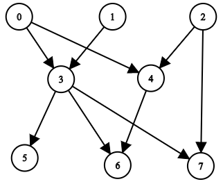
Input: n = 8, edgeList = [[0,3],[0,4],[1,3],[2,4],[2,7],[3,5],[3,6],[3,7],[4,6]]
Output: [[],[],[],[0,1],[0,2],[0,1,3],[0,1,2,3,4],[0,1,2,3]]
Explanation:
The above diagram represents the input graph.
Nodes 0, 1, and 2 do not have any ancestors.
Node 3 has two ancestors 0 and 1.
Node 4 has two ancestors 0 and 2.
Node 5 has three ancestors 0, 1, and 3.
Node 6 has five ancestors 0, 1, 2, 3, and 4.
Node 7 has four ancestors 0, 1, 2, and 3.
Example 2:
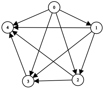
Input: n = 5, edgeList = [[0,1],[0,2],[0,3],[0,4],[1,2],[1,3],[1,4],[2,3],[2,4],[3,4]]
Output: [[],[0],[0,1],[0,1,2],[0,1,2,3]]
Explanation:
The above diagram represents the input graph.
Node 0 does not have any ancestor.
Node 1 has one ancestor 0.
Node 2 has two ancestors 0 and 1.
Node 3 has three ancestors 0, 1, and 2.
Node 4 has four ancestors 0, 1, 2, and 3.
Constraints:
1 <= n <= 10000 <= edges.length <= min(2000, n * (n - 1) / 2)edges[i].length == 20 <= from_i, to_i <= n - 1from_i != to_iThere are no duplicate edges.
The graph is directed and acyclic.
Approach 1: Depth-First Search (DFS) with Ancestor Propagation
Understanding the Core Idea
The central concept of this solution is to leverage a depth-first search (DFS) approach to propagate ancestor information through a Directed Acyclic Graph (DAG). This method efficiently builds a complete ancestor list for each node by traversing the graph structure.
Graph Representation: The solution uses an adjacency list to represent the DAG, which allows for efficient lookup of a node's direct children.
Ancestor Propagation: Instead of finding ancestors for each node independently, the algorithm propagates each node as an ancestor to all of its descendants.
Recursive Traversal: A depth-first search is implemented recursively to ensure all descendants of a node receive the ancestor information.
Code Walkthrough
Initialization:
direct_children = defaultdict(list) ancestors: List[List[int]] = [[] for _ in range(n)]The code initializes two key data structures:
direct_children: Adefaultdictto store the adjacency list representation of the graph.ancestors: A list of lists to store the ancestors for each node.
Building the Adjacency List:
for parent, child in edges: direct_children[parent].append(child)This loop processes the input edges to construct the adjacency list. For each edge, it adds the child node to the list of direct children for the parent node.
Defining the Propagation Function:
def propagate_ancestor(current_ancestor: int, current_node: int): for child in direct_children[current_node]: if (not ancestors[child] or ancestors[child][-1] != current_ancestor): ancestors[child].append(current_ancestor) propagate_ancestor(current_ancestor, child)This helper function recursively propagates ancestry information:
It iterates through all direct children of the current node.
For each child, it checks if the current ancestor needs to be added (avoiding duplicates).
If the child has no ancestors or the last ancestor is not the current ancestor, it adds the current ancestor.
The last check works because we iterate in ascending order, ensuring the current ancestor is always the latest one.
If needed, it adds the ancestor and recursively calls itself for the child node.
Initiating Ancestor Propagation:
for node in range(n): propagate_ancestor(node, node)This loop initiates the propagation process for each node in the graph. Each node is considered as its own ancestor to start the propagation.
Result Return:
return ancestorsThe function returns the
ancestorslist, which now contains the complete list of ancestors for each node.
Complexity Analysis
Time Complexity:
, where is the number of nodes and is the number of edges. This is because: The outer loop runs
times, once for each node. For each iteration, the
propagate_ancestorfunction potentially traverses all descendants of the node, which in the worst case could be all nodes and edges in the graph.
Space Complexity:
, where is the number of nodes and is the number of edges. This is because: The
direct_childrenadjacency list takesspace. The
ancestorslist takesspace in the worst case, where each node could potentially have all other nodes as ancestors. The recursion stack in the worst case could go up to
depth.
Example
Input:
Step-by-Step Walkthrough:
Initialization:
Initialize
direct_childrenas an empty defaultdict(list).Create
ancestorsas a list of eight empty lists:[[], [], [], [], [], [], [], []].
Building the Adjacency List:
Iterate through each edge in
edges:For [0, 3]: Add 3 to
direct_children[0]For [0, 4]: Add 4 to
direct_children[0]For [1, 3]: Add 3 to
direct_children[1]For [2, 4]: Add 4 to
direct_children[2]For [2, 7]: Add 7 to
direct_children[2]For [3, 5]: Add 5 to
direct_children[3]For [3, 6]: Add 6 to
direct_children[3]For [3, 7]: Add 7 to
direct_children[3]For [4, 6]: Add 6 to
direct_children[4]
Final
direct_children: {0: [3, 4], 1: [3], 2: [4, 7], 3: [5, 6, 7], 4: [6]}Main Loop: Propagating Ancestors:
Iterate through each node from 0 to 7:
Node 0:
Call
propagate_ancestor(0, 0)Propagate to children 3 and 4:
For child 3: Add 0 to
ancestors[3], then recursively propagateAdd 0 to
ancestors[5],ancestors[6], andancestors[7]
For child 4: Add 0 to
ancestors[4], then recursively propagateAdd 0 to
ancestors[6](already present, so skip)
Node 1:
Call
propagate_ancestor(1, 1)Propagate to child 3:
Add 1 to
ancestors[3], then recursively propagateAdd 1 to
ancestors[5],ancestors[6], andancestors[7]
Node 2:
Call
propagate_ancestor(2, 2)Propagate to children 4 and 7:
For child 4: Add 2 to
ancestors[4], then recursively propagateAdd 2 to
ancestors[6]
For child 7: Add 2 to
ancestors[7]
Node 3:
Call
propagate_ancestor(3, 3)Propagate to children 5, 6, and 7:
Add 3 to
ancestors[5],ancestors[6], andancestors[7]
Node 4:
Call
propagate_ancestor(4, 4)Propagate to child 6:
Add 4 to
ancestors[6]
Nodes 5, 6, and 7:
Call
propagate_ancestorfor each, but they have no children, so no further propagation occurs
Visual Aid: Iteration Summary
Node
Ancestors
Direct Children
0
[]
[3, 4]
1
[]
[3]
2
[]
[4, 7]
3
[0, 1]
[5, 6, 7]
4
[0, 2]
[6]
5
[0, 1, 3]
[]
6
[0, 1, 2, 3, 4]
[]
7
[0, 1, 2, 3]
[]
Result Calculation/Final Steps:
The
ancestorslist now contains the final result:[[], [], [], [0, 1], [0, 2], [0, 1, 3], [0, 1, 2, 3, 4], [0, 1, 2, 3]]This list represents the ancestors of each node in ascending order:
Node 0: No ancestors
Node 1: No ancestors
Node 2: No ancestors
Node 3: Ancestors are 0 and 1
Node 4: Ancestors are 0 and 2
Node 5: Ancestors are 0, 1, and 3
Node 6: Ancestors are 0, 1, 2, 3, and 4
Node 7: Ancestors are 0, 1, 2, and 3
The function returns this
ancestorslist as the final result.
Approach 2: Depth-First Search (DFS) with Memoization
Understanding the Core Idea
The central concept of this solution is to leverage a depth-first search (DFS) approach combined with memoization to efficiently compute and store the ancestors of each node in a Directed Acyclic Graph (DAG). This method builds a complete ancestor list for each node by traversing the graph structure upwards and caching results to avoid redundant computations.
Reverse Graph Representation: The solution uses a reverse adjacency list (
direct_parents) to represent the DAG, allowing for efficient upward traversal from a node to its parents.Recursive Memoization: A depth-first search is implemented recursively with memoization, ensuring that each node's ancestors are computed only once and then cached for future use.
Set Operations: The use of sets for intermediate computations allows for efficient union operations and automatic elimination of duplicates.
Code Walkthrough
Initialization:
direct_parents = defaultdict(list) ancestors = [[] for _ in range(n)]The code initializes two key data structures:
direct_parents: A defaultdict to store the reverse adjacency list of the graph.ancestors: A list of lists to store the final sorted ancestors for each node.
Building the Reverse Adjacency List:
for parent, child in edges: direct_parents[child].append(parent)This loop processes the input edges to construct the reverse adjacency list. For each edge, it adds the parent node to the list of direct parents for the child node.
Defining the Recursive Ancestor-Finding Function:
def find_all_ancestors(node: int) -> set: if ancestors[node]: return set(ancestors[node]) result = set() for parent in direct_parents[node]: result.update(find_all_ancestors(parent)) result.update(direct_parents[node]) ancestors[node] = list(result) return resultThis helper function recursively finds and memoizes all ancestors of a given node:
It first checks if the ancestors for the node are already computed (memoization).
If not, it recursively computes the ancestors of each parent and updates the result set.
It then adds the direct parents to the result set.
Finally, it caches the result in the
ancestorslist and returns the set.
Initiating Ancestor Computation:
for node in range(n): if not ancestors[node]: find_all_ancestors(node)This loop initiates the ancestor computation process for each node in the graph that hasn't been processed yet.
Sorting the Ancestors:
for node in range(n): ancestors[node].sort()This step sorts the ancestors for each node in ascending order, as required by the problem statement.
Result Return:
return ancestorsThe function returns the
ancestorslist, which now contains the complete, sorted list of ancestors for each node.
Complexity Analysis
Time Complexity:
, where is the number of nodes and is the number of edges. This is because: In the worst case, each node might need to traverse all edges to find its ancestors.
The sorting step for each node takes
time, but this is dominated by the traversal in sparse graphs. The memoization ensures that each node's ancestors are computed only once.
Space Complexity:
, where is the number of nodes and is the number of edges. This is because: The
direct_parentsadjacency list takesspace. The
ancestorslist takesspace in the worst case, where each node could potentially have all other nodes as ancestors. The recursion stack in the worst case could go up to
depth. The set used for intermediate computations can take up to
space for each recursive call.
Example
Input:
Step-by-Step Walkthrough:
Initialization:
Initialize
direct_parentsas an empty defaultdict(list).Create
ancestorsas a list of eight empty lists:[[], [], [], [], [], [], [], []].
Building the Reverse Adjacency List:
Iterate through each edge in
edges:For [0, 3]: Add 0 to
direct_parents[3]For [0, 4]: Add 0 to
direct_parents[4]For [1, 3]: Add 1 to
direct_parents[3]For [2, 4]: Add 2 to
direct_parents[4]For [2, 7]: Add 2 to
direct_parents[7]For [3, 5]: Add 3 to
direct_parents[5]For [3, 6]: Add 3 to
direct_parents[6]For [3, 7]: Add 3 to
direct_parents[7]For [4, 6]: Add 4 to
direct_parents[6]
Final
direct_parents: {3: [0, 1], 4: [0, 2], 7: [2, 3], 5: [3], 6: [3, 4]}Main Loop: Computing Ancestors:
Iterate through each node from 0 to 7:
Node 0:
Call
find_all_ancestors(0)No direct parents, return empty set
ancestors[0]remains[]
Node 1:
Call
find_all_ancestors(1)No direct parents, return empty set
ancestors[1]remains[]
Node 2:
Call
find_all_ancestors(2)No direct parents, return empty set
ancestors[2]remains[]
Node 3:
Call
find_all_ancestors(3)Direct parents: [0, 1]
Recursively call for parent 0 (returns an empty set)
Recursively call for parent 1 (returns an empty set)
Add direct parents [0, 1] to result
Set
ancestors[3] = [0, 1]
Node 4:
Call
find_all_ancestors(4)Direct parents: [0, 2]
Recursively call for parent 0 (returns an empty set)
Recursively call for parent 2 (returns an empty set)
Add direct parents [0, 2] to result
Set
ancestors[4] = [0, 2]
Node 5:
Call
find_all_ancestors(5)Direct parents: [3]
Recursively call for parent 3 (returns {0, 1})
Add direct parent 3 to result
Set
ancestors[5] = [0, 1, 3]
Node 6:
Call
find_all_ancestors(6)Direct parents: [3, 4]
Recursively call for parent 3 (returns {0, 1})
Recursively call for parent 4 (returns {0, 2})
Add direct parents [3, 4] to result
Set
ancestors[6] = [0, 1, 2, 3, 4]
Node 7:
Call
find_all_ancestors(7)Direct parents: [2, 3]
Recursively call for parent 2 (returns an empty set)
Recursively call for parent 3 (returns {0, 1})
Add direct parents [2, 3] to result
Set
ancestors[7] = [0, 1, 2, 3]
Sorting Ancestors:
For each node, sort its list of ancestors:
Node 0: [] (no change)
Node 1: [] (no change)
Node 2: [] (no change)
Node 3: [0, 1] (already sorted)
Node 4: [0, 2] (already sorted)
Node 5: [0, 1, 3] (already sorted)
Node 6: [0, 1, 2, 3, 4] (already sorted)
Node 7: [0, 1, 2, 3] (already sorted)
Visual Aid: Iteration Summary
Node
Ancestors
Direct Parents
0
[]
[]
1
[]
[]
2
[]
[]
3
[0, 1]
[0, 1]
4
[0, 2]
[0, 2]
5
[0, 1, 3]
[3]
6
[0, 1, 2, 3, 4]
[3, 4]
7
[0, 1, 2, 3]
[2, 3]
Result Calculation/Final Steps:
The
ancestorslist now contains the final result:[[], [], [], [0, 1], [0, 2], [0, 1, 3], [0, 1, 2, 3, 4], [0, 1, 2, 3]]This list represents the sorted ancestors of each node:
Node 0: No ancestors
Node 1: No ancestors
Node 2: No ancestors
Node 3: Ancestors are 0 and 1
Node 4: Ancestors are 0 and 2
Node 5: Ancestors are 0, 1, and 3
Node 6: Ancestors are 0, 1, 2, 3, and 4
Node 7: Ancestors are 0, 1, 2, and 3
The function returns this
ancestorslist as the final result.
Approach 3: Breadth-First Search (BFS) with Topological Sorting
Understanding the Core Idea
The central concept of this solution is to combine a breadth-first search (BFS) approach with topological sorting to efficiently compute the ancestors of each node in a Directed Acyclic Graph (DAG). This method processes nodes in an order that ensures all ancestors are computed before they're needed, allowing for a single pass through the graph.
Graph Representation: The solution uses an adjacency list (
direct_children) to represent the DAG, facilitating efficient traversal of child nodes.Topological Sorting: By using in-degree counting and a queue-based approach, the algorithm processes nodes in topological order, ensuring that a node is only processed after all its ancestors have been computed.
Set Operations: The use of sets for storing ancestors allows for efficient update operations and automatic deduplication.
Code Walkthrough
Initialization:
direct_children = defaultdict(list) ancestors = [set() for _ in range(n)] in_degree = [0] * nThe code initializes three key data structures:
direct_children: A defaultdict to store the adjacency list of the graph.ancestors: A list of sets to store the ancestors for each node.in_degree: An array to keep track of the number of incoming edges for each node.
Building the Graph and Initial Ancestor Sets:
for parent, child in edges: direct_children[parent].append(child) ancestors[child].add(parent) in_degree[child] += 1This loop processes the input edges to:
Construct the adjacency list (
direct_children).Initialize the direct ancestors for each node.
Calculate the in-degree for each node.
Initializing the Queue for Topological Sort:
queue = deque(node for node in range(n) if in_degree[node] == 0)This step identifies all nodes with no incoming edges (in-degree of 0) and adds them to the queue. These nodes serve as the starting points for the topological traversal.
Processing Nodes in Topological Order:
while queue: current_node = queue.popleft() for child_node in direct_children[current_node]: ancestors[child_node].update(ancestors[current_node]) in_degree[child_node] -= 1 if in_degree[child_node] == 0: queue.append(child_node)This is the core BFS loop that processes nodes in topological order:
It pops a node from the queue and processes all its children.
For each child, it updates its ancestor set by adding all ancestors of the current node.
It decrements the in-degree of the child node.
If a child's in-degree becomes 0, it's added to the queue for processing.
Result Preparation and Return:
return [sorted(node_ancestors) for node_ancestors in ancestors]This final step converts the sets of ancestors to sorted lists, as required by the problem statement, and returns the result.
Complexity Analysis
Time Complexity:
in the worst case, where is the number of nodes and is the number of edges. This is because: Building the initial graph structure takes
time. In the worst case (e.g., a chain structure), each node might accumulate all previous nodes as ancestors, leading to
total ancestors across all nodes. Sorting these large ancestor lists takes
time per node, resulting in for all nodes. The BFS traversal itself processes each edge once, taking
time.
Space Complexity:
, which simplifies to , where is the number of nodes and is the number of edges. This is because: The
ancestorslist of sets can take up tospace in the worst case, where each node has all other nodes as ancestors. The
direct_childrenadjacency list takesspace. The
in_degreearray and queue takespace.
It's worth noting that while this worst-case time complexity appears higher than the previous approaches, this algorithm often performs better in practice for many graph structures, especially sparse graphs, due to its non-recursive nature and efficient set operations.
Example
Input:
Step-by-Step Walkthrough:
Initialization:
Initialize
direct_childrenas an empty defaultdict(list).Create
ancestorsas a list of eight empty sets:[set(), set(), set(), set(), set(), set(), set(), set()].Initialize
in_degreeas a list of 8 zeros:[0, 0, 0, 0, 0, 0, 0, 0].
Building Graph Data Structures:
Iterate through each edge in
edges:For [0, 3]: Add 3 to
direct_children[0], add 0 toancestors[3], incrementin_degree[3]For [0, 4]: Add 4 to
direct_children[0], add 0 toancestors[4], incrementin_degree[4]For [1, 3]: Add 3 to
direct_children[1], add 1 toancestors[3], incrementin_degree[3]For [2, 4]: Add 4 to
direct_children[2], add 2 toancestors[4], incrementin_degree[4]For [2, 7]: Add 7 to
direct_children[2], add 2 toancestors[7], incrementin_degree[7]For [3, 5]: Add 5 to
direct_children[3], add 3 toancestors[5], incrementin_degree[5]For [3, 6]: Add 6 to
direct_children[3], add 3 toancestors[6], incrementin_degree[6]For [3, 7]: Add 7 to
direct_children[3], add 3 toancestors[7], incrementin_degree[7]For [4, 6]: Add 6 to
direct_children[4], add 4 toancestors[6], incrementin_degree[6]
Final state:
direct_children: {0: [3, 4], 1: [3], 2: [4, 7], 3: [5, 6, 7], 4: [6]}ancestors: [set(), set(), set(), {0, 1}, {0, 2}, {3}, {3, 4}, {2, 3}]in_degree: [0, 0, 0, 2, 2, 1, 2, 2]
Initializing Queue:
Add nodes with in-degree 0 to the queue: [0, 1, 2]
Processing Nodes in Topological Order:
Process Node 0:
Current queue: [1, 2]
Children: [3, 4]
For child 3:
Update
ancestors[3]to {0, 1}Decrement
in_degree[3]to 1
For child 4:
Update
ancestors[4]to {0, 2}Decrement
in_degree[4]to 1
Process Node 1:
Current queue: [2]
Children: [3]
For child 3:
Update
ancestors[3]to {0, 1}Decrement
in_degree[3]to 0Add 3 to queue: [2, 3]
Process Node 2:
Current queue: [3]
Children: [4, 7]
For child 4:
Update
ancestors[4]to {0, 2}Decrement
in_degree[4]to 0Add 4 to queue: [3, 4]
For child 7:
Update
ancestors[7]to {2, 3}Decrement
in_degree[7]to 1
Process Node 3:
Current queue: [4]
Children: [5, 6, 7]
For child 5:
Update
ancestors[5]to {0, 1, 3}Decrement
in_degree[5]to 0Add 5 to queue: [4, 5]
For child 6:
Update
ancestors[6]to {0, 1, 3, 4}Decrement
in_degree[6]to 1
For child 7:
Update
ancestors[7]to {0, 1, 2, 3}Decrement
in_degree[7]to 0Add 7 to queue: [4, 5, 7]
Process Node 4:
Current queue: [5, 7]
Children: [6]
For child 6:
Update
ancestors[6]to {0, 1, 2, 3, 4}Decrement
in_degree[6]to 0Add 6 to queue: [5, 7, 6]
Process Node 5:
Current queue: [7, 6]
No children, hence we do nothing
Process Node 7:
Current queue: [6]
No children, hence we do nothing
Process Node 6:
Current queue: []
No children, hence we do nothing
Sorting Ancestors:
For each node, convert its set of ancestors to a sorted list:
Node 0: [] (empty set to empty list)
Node 1: [] (empty set to empty list)
Node 2: [] (empty set to empty list)
Node 3: [0, 1]
Node 4: [0, 2]
Node 5: [0, 1, 3]
Node 6: [0, 1, 2, 3, 4]
Node 7: [0, 1, 2, 3]
Visual Aid: Iteration Summary
Processed Node
Ancestors
Direct Children
Final In-Degree
0
set()
[3, 4]
0
1
set()
[3]
0
2
set()
[4, 7]
0
3
{0, 1}
[5, 6, 7]
0
4
{0, 2}
[6]
0
5
{0, 1, 3}
[]
0
7
{0, 1, 2, 3}
[]
0
6
{0, 1, 2, 3, 4}
[]
0
Result Calculation/Final Steps:
The
ancestorslist now contains the final result:[[], [], [], [0, 1], [0, 2], [0, 1, 3], [0, 1, 2, 3, 4], [0, 1, 2, 3]]This list represents the sorted ancestors of each node:
Node 0: No ancestors
Node 1: No ancestors
Node 2: No ancestors
Node 3: Ancestors are 0 and 1
Node 4: Ancestors are 0 and 2
Node 5: Ancestors are 0, 1, and 3
Node 6: Ancestors are 0, 1, 2, 3, and 4
Node 7: Ancestors are 0, 1, 2, and 3
The function returns this
ancestorslist as the final result.
June 30 -> 1579. Remove Max Number of Edges to Keep Graph Fully Traversable
Alice and Bob have an undirected graph of n nodes and three types of edges:
Type 1: Can be traversed by Alice only.
Type 2: Can be traversed by Bob only.
Type 3: Can be traversed by both Alice and Bob.
Given an array edges where edges[i] = [type_i, u_i, v_i] represents a bidirectional edge of type type_i between nodes u_i and v_i, find the maximum number of edges you can remove so that after removing the edges, the graph can still be fully traversed by both Alice and Bob. The graph is fully traversed by Alice and Bob if starting from any node, they can reach all other nodes.
Return the maximum number of edges you can remove, or return -1 if Alice and Bob cannot fully traverse the graph.
Example 1:
Input: n = 4, edges = [[3,1,2],[3,2,3],[1,1,3],[1,2,4],[1,1,2],[2,3,4]]
Output: 2
Explanation: If we remove the two edges [1,1,2] and [1,1,3]. The graph will still be fully traversable by Alice and Bob. Removing any additional edge will not make it so. So the maximum number of edges we can remove is 2.
Example 2:
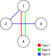
Input: n = 4, edges = [[3,1,2],[3,2,3],[1,1,4],[2,1,4]]
Output: 0
Explanation: Notice that removing any edge will not make the graph fully traversable by Alice and Bob.
Example 3:
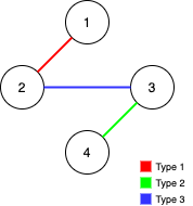
Input: n = 4, edges = [[3,2,3],[1,1,2],[2,3,4]]
Output:-1
Explanation: In the current graph, Alice cannot reach node 4 from the other nodes. Likewise, Bob cannot reach 1. Therefore, it's impossible to make the graph fully traversable.
Constraints:
1 <= n <= 10^51 <= edges.length <= min(10^5, 3 * n * (n - 1) / 2)edges[i].length == 31 <= typei <= 31 <= u_i < v_i <= nAll tuples
(type_i, u_i, v_i)are distinct.
Approach 1: Union-Find with Two-Pass Edge Processing
Understanding the Core Idea
The central concept of this solution is to leverage the Union-Find data structure to efficiently track connected components for both Alice and Bob separately. The solution processes edges in two passes, prioritizing shared (type 3) edges to potentially maximize removable edges.
Dual Union-Find Structures: The solution uses two separate Union-Find structures, one for Alice and one for Bob, to track their respective traversable paths independently.
Two-Pass Edge Processing: Edges are processed in two passes - first type 3 (shared) edges, then type 1 ( Alice-only) and type 2 (Bob-only) edges. This prioritization helps maximize the number of removable edges.
Essential Edge Tracking: The solution keeps count of "essential" edges that must be kept for full traversal, which is used to calculate the maximum removable edges.
Code Walkthrough
Initialization:
alice_uf = UnionFind(size=n, offset=1) bob_uf = UnionFind(size=n, offset=1) essential_edges = 0Two
UnionFindstructures are initialized, one for Alice and one for Bob. Theoffset=1is used because node numbering starts from 1.essential_edgeskeeps track of edges that must be kept.First Pass - Processing Type 3 Edges:
for edge_type, u, v in edges: if edge_type == 3: essential_edges += alice_uf.union(u, v) | bob_uf.union(u, v) if alice_uf.is_single_component(): return len(edges) - essential_edgesThis loop processes all type 3 edges first. The
unionoperation is performed for both Alice and Bob, and the result is OR'ed to incrementessential_edgesif either union was successful. If Alice's graph becomes fully connected, we can immediately return the result as Bob's graph will also be fully connected.Second Pass - Processing Type 1 and Type 2 Edges:
for edge_type, u, v in edges: if edge_type == 1: if alice_uf.union(u, v): essential_edges += 1 elif edge_type == 2: if bob_uf.union(u, v): essential_edges += 1 if alice_uf.is_single_component() and bob_uf.is_single_component(): return len(edges) - essential_edgesThis loop processes type 1 (Alice-only) and type 2 (Bob-only) edges. It performs the union operation and increments
essential_edgesif the union was successful. After each edge, it checks if both graphs are fully connected.Result Calculation/Return:
return -1 # Full traversal is not possible for both Alice and BobIf the function reaches this point, it means full traversal is not possible for both Alice and Bob, so it returns -1.
Complexity Analysis
Time Complexity:
, where is the number of nodes, is the number of edges, and is the inverse Ackermann function. This is because each Union-Find operation (union and find) takes amortized
time, and we perform at most such operations (once for each edge in each pass). The inverse Ackermann function
grows extremely slowly and is effectively constant for all practical values of .
Space Complexity:
, where is the number of nodes. This is due to the two UnionFind data structures, each storing parent and rank information for
nodes. The space used is independent of the number of edges, making it efficient for dense graphs.
Example
Input:
Step-by-Step Walkthrough:
Initialization:
Initialize two UnionFind data structures:
alice_ufandbob_uf, both with size 4 and offset 1.Set
essential_edgesto 0.
First Pass: Processing Type 3 Edges
Iteration 1:
Process edge [3, 1, 2]
For both Alice and Bob:
Union nodes 1 and 2
This is a new connection, so increment
essential_edgesto 1
Check if Alice's graph is fully connected (it's not)
Iteration 2:
Process edge [3, 2, 3]
For both Alice and Bob:
Union nodes 2 and 3
This is a new connection, so increment
essential_edgesto 2
Check if Alice's graph is fully connected (it's not)
Second Pass: Processing Type 1 and Type 2 Edges
Iteration 3:
Process edge [1, 1, 3]
For Alice only:
Attempt to union nodes 1 and 3
They are already connected, so no change to
essential_edges
Check if both graphs are fully connected (they're not)
Iteration 4:
Process edge [1, 2, 4]
For Alice only:
Union nodes 2 and 4
This is a new connection, so increment
essential_edgesto 3
Check if both graphs are fully connected (Alice's is, Bob's isn't)
Iteration 5:
Process edge [1, 1, 2]
For Alice only:
Attempt to union nodes 1 and 2
They are already connected, so no change to
essential_edges
Check if both graphs are fully connected (Alice's is, Bob's isn't)
Iteration 6:
Process edge [2, 3, 4]
For Bob only:
Union nodes 3 and 4
This is a new connection, so increment
essential_edgesto 4
Check if both graphs are fully connected (they are)
Visual Aid:
Here's a table summarizing the edge processing:
Edge #
Type
U
V
Alice Union
Bob Union
Essential Edges
1
3
1
2
True
True
1
2
3
2
3
True
True
2
3
1
1
3
False
-
2
4
1
2
4
True
-
3
5
1
1
2
False
-
3
6
2
3
4
-
True
4
Result Calculation:
Total number of edges: 6
Number of essential edges: 4
Maximum number of edges that can be removed: 6 - 4 = 2
The algorithm determines that two edges can be removed while still allowing both Alice and Bob to fully traverse the graph. These removable edges are the ones that didn't result in new connections: [1, 1, 3] and [1, 1, 2].