June 2024 Weekly Exercises
Week 1 -> 1940. Longest Common Subsequence Between Sorted Arrays
Given an array of integer arrays arrays where each arrays[i] is sorted in strictly increasing order, return an integer array representing the longest common subsequence between all the arrays.
A subsequence is a sequence that can be derived from another sequence by deleting some elements (possibly none) without changing the order of the remaining elements.
Example 1:
Input: arrays = [[1,3,4], [1,4,7,9]]
Output: [1,4]
Explanation: The longest common subsequence in the two arrays is [1,4].
Example 2:
Input: arrays = [[2,3,6,8], [1,2,3,5,6,7,10], [2,3,4,6,9]]
Output: [2,3,6]
Explanation: The longest common subsequence in all three arrays is [2,3,6].
Example 3:
Input: arrays = [[1,2,3,4,5], [6,7,8]]
Output: []
Explanation: There is no common subsequence between the two arrays.
Constraints:
2 <= arrays.length <= 1001 <= arrays[i].length <= 1001 <= arrays[i][j] <= 100arrays[i]is sorted in strictly increasing order.
Approach 1: Binary Search
Understanding the Core Idea
The core idea of this solution is to optimize the search for common elements in multiple sorted arrays by focusing on the smallest array. It leverages binary search to efficiently check if elements from the smallest array exist in all other arrays. This approach reduces the overall search space and time complexity compared to a naive brute-force method.
Binary Search: Utilizes the fact that the arrays are sorted to perform efficient logarithmic-time searches for elements.
Smallest Array Focus: By iterating through the smallest array, we minimize the number of elements that need to be checked across all arrays, leading to a potential performance improvement.
Common Subsequence Construction: An element is added to the longest common subsequence (LCS) only if it's found in all other arrays, ensuring the result is a valid subsequence shared by all.
Code Walkthrough
Initialization:
Finds the
smallest_arrayusing theminfunction with a key based on array length.Removes the
smallest_arrayfrom thearrayslist to avoid redundant searches.Initializes an empty list
common_subsequencesto store the LCS.
Helper Function (
binary_search):This function takes an array
arrayand a target numbernum.It uses
bisect_leftto find the insertion point fornuminarraywhile maintaining sorted order.If
numis found at the insertion point, it returnsTrue; otherwise, it returnsFalse.
Main Loop (Finding Common Elements):
Iterates through each
numin thesmallest_array.For each
num:A generator expression checks if
numis present in all remaining arrays usingbinary_search.The
allfunction checks if all results from the generator areTrue.If
numis found in all arrays, it's added tocommon_subsequences.
Return Result:
Returns the
common_subsequenceslist, representing the longest common subsequence found.
Complexity Analysis
Time Complexity:
, where: is the number of elements in the smallest array. is the total number of arrays. is the average length of the arrays.
The nested loops dominate the time complexity. The outer loop iterates through the smallest array (n iterations), and the inner loop implicitly iterates through all remaining arrays (m-1 iterations) within the generator expression. For each element in the smallest array, we perform a binary search in each of the other arrays, with an average time complexity of O(log(k)).
Space Complexity:
, where is the length of the longest common subsequence. The main space usage is due to storing the elements of the LCS in the
common_subsequenceslist. The space used by thebinary_searchfunction is constant.
Example
Input: arrays = [[2, 3, 6, 8], [1, 2, 3, 5, 6, 7, 10], [2, 3, 4, 6, 9]]
Step-by-Step Walkthrough:
Initialization:
The function prints the initial
arraysinput:[[2, 3, 6, 8], [1, 2, 3, 5, 6, 7, 10], [2, 3, 4, 6, 9]]An empty list
common_subsequencesis initialized to store the LCS.
Identifying Smallest Array:
The function identifies
[2, 3, 6, 8]as the smallest array.This array is removed from the
arrayslist, leaving[[1, 2, 3, 5, 6, 7, 10], [2, 3, 4, 6, 9]].
Main Loop (Finding Common Elements): The function iterates through the smallest array,
[2, 3, 6, 8].Iteration 1:
num= 2binary_searchis used to check for the presence of2in the remaining arrays:binary_search([1, 2, 3, 5, 6, 7, 10], 2)returnsTrue.binary_search([2, 3, 4, 6, 9], 2)returnsTrue.
Since
2is found in both remaining arrays, it is added tocommon_subsequences:[2]
Iteration 2:
num= 3binary_search([1, 2, 3, 5, 6, 7, 10], 3)returnsTrue.binary_search([2, 3, 4, 6, 9], 3)returnsTrue.'3' is added to
common_subsequences:[2, 3]
Iteration 3:
num= 6binary_search([1, 2, 3, 5, 6, 7, 10], 6)returnsTrue.binary_search([2, 3, 4, 6, 9], 6)returnsTrue.'6' is added to
common_subsequences:[2, 3, 6]
Iteration 4:
num= 8binary_search([1, 2, 3, 5, 6, 7, 10], 8)returnsFalse.Since '8' is not found in all arrays, the loop moves to the next iteration without updating
common_subsequences.
Iteration Summary:
Iteration
numcommon_subsequences1
2
[2]
2
3
[2, 3]
3
6
[2, 3, 6]
4
8
[2, 3, 6]
Result Calculation/Final Steps:
The function reaches the end of the loop, and the final
common_subsequencesis[2, 3, 6]. This is returned as the longest common subsequence among the input arrays.
Approach 2: Two Pointer Technique
Understanding the Core Idea
The core idea of this solution is to use a two-pointer technique, similar to merging sorted arrays, to iteratively refine the longest common subsequence (LCS). It starts by assuming the first array is the initial LCS. Then, for each later array, it compares elements with the current LCS using two pointers, keeping only the elements that match in a new subsequence. This new subsequence then becomes the LCS for the next comparison.
Two-Pointer Technique: This technique enables efficient traversal and comparison of sorted arrays, avoiding nested loops and reducing time complexity.
Iterative Refinement: The LCS is continuously updated, ensuring that only the longest common elements persist across all arrays.
Sorted Property: The algorithm leverages the sorted nature of the arrays, allowing for linear time complexity through pointer advancement based on element comparisons.
Code Walkthrough
Initialization:
common_subsequencesis initialized with the first array in thearrayslist, representing the initial LCS.
Iterative Refinement Loop:
The
forloop iterates through each array inarraysstarting from the second array.new_subsequenceis created to store the potential LCS found in the current iteration.Two pointers,
array_index(for the current array) andcommon_subseq_index(for the currentcommon_subsequences) are initialized to 0.The lengths of the current array and the current
common_subsequencesare stored inarray_lengthandcommon_subseq_length, respectively.
Two-Pointer Comparison:
The
whileloop continues as long as both pointers are within the bounds of their respective lists.The following cases are handled inside the loop:
Match: If the elements at the current indices match, the element is appended to
new_subsequence, and both pointers are incremented.Element in
arrayis Smaller: Thearray_indexis incremented to find a potential match further in the array.Element in
common_subsequencesis Smaller: Thecommon_subseq_indexis incremented to find a potential match further in the common subsequence.
Update and Continue:
After processing an array,
common_subsequencesis updated withnew_subsequence, which now represents the longest common subsequence found so far.The process repeats for the next array in
arrays.
Return Result:
After all arrays are processed, the final
common_subsequencesis returned, representing the longest common subsequence between all the input arrays.
Complexity Analysis
Time Complexity:
, where is the length of the input string. This is because each character is processed once in the main loop, and while the inner while loop may seem to add additional iterations, each character is removed from the set at most once across all iterations.
Space Complexity:
, because the set window_charsstores at most 26 characters (the size of the lowercase English alphabet). While this could be written aswhere is the size of the alphabet, since is fixed at 26, it's considered constant space.
Example
Input: arrays = [[2, 3, 6, 8], [1, 2, 3, 5, 6, 7, 10], [2, 3, 4, 6, 9]]
Step-by-Step Walkthrough:
Initialization:
common_subsequencesis initialized with the first array:[2, 3, 6, 8].This represents the initial longest common subsequence (LCS), as it's the only one considered so far.
Main Loop (Iterative Refinement of Common Subsequence):
Iteration 1:
We compare
common_subsequences(currently[2, 3, 6, 8]) with the second array:[1, 2, 3, 5, 6, 7, 10].Initially,
array_index = 0,common_subseq_index = 0Comparing
2(fromcommon_subsequences) and1(from the second array):1is smaller, so we move to the next element in the second array (array_index = 1).Comparing
2and2: Match found! We add2tonew_subsequenceand advance both pointers.Comparing
3and3: Match found! We add3tonew_subsequenceand advance both pointers.Comparing
6and5:5is smaller, so we move to the next element in the second array.Comparing
6and6: Match found! We add6tonew_subsequenceand advance both pointers.Comparing
8and7:7is smaller, so we move to the next element in the second array.Comparing
8and10:8is smaller, but we've reached the end ofcommon_subsequences. The loop terminates.
new_subsequenceis now[2, 3, 6]. This becomes the newcommon_subsequencesfor the next iteration.
Iteration 2:
We compare the updated
common_subsequences([2, 3, 6]) with the third array:[2, 3, 4, 6, 9].Initially,
array_index = 0,common_subseq_index = 0Comparing
2and2: Match found! We add2tonew_subsequenceand advance both pointers.Comparing
3and3: Match found! We add3tonew_subsequenceand advance both pointers.Comparing
6and4:4is smaller, so we move to the next element in the third array.Comparing
6and6: Match found! We add6tonew_subsequenceand advance both pointers.The loop terminates as we reach the end of 'common_subsequences.'
new_subsequenceis now[2, 3, 6]. This is the final LCS.
Loop Termination: The loop terminates after iterating through all arrays in the input.
Iteration Summary:
Iteration
Array Compared
Resulting Common Subsequence
1
[1, 2, 3, 5, 6, 7, 10]
[2, 3, 6]
2
[2, 3, 4, 6, 9]
[2, 3, 6]
Result Calculation/Final Steps:
After the loop, the final
common_subsequencesis[2, 3, 6]. This is returned as the longest common subsequence across all input arrays.
Complexity Analysis
Time Complexity:
, where: is the total number of arrays. is the average length of the arrays.
In the worst case, the algorithm might iterate through all elements of each array once for comparison, resulting in linear time complexity with respect to the total number of elements.
Space Complexity:
, where is the maximum length among the input arrays. The algorithm uses a
new_subsequencelist to store the potential LCS in each iteration. The maximum size of this list would be the maximum length among the input arrays. Thecommon_subsequenceslist may also hold up to K elements at any given time.
Week 2 -> 2083. Substrings That Begin and End With the Same Letter
You are given a 0-indexed string s consisting of only lowercase English letters. Return the number of substrings in s that begin and end with the same character.
A substring is a contiguous non-empty sequence of characters within a string.
Example 1:
Input: s = "abcba"
Output: 7
Explanation:
The substrings of length 1 that start and end with the same letter are: "a", "b", "c", "b", and "a".
The substring of length 3 that starts and ends with the same letter is: "bcb".
The substring of length 5 that starts and ends with the same letter is: "abcba".
Example 2:
Input: s = "abacad"
Output: 9
Explanation:
The substrings of length 1 that start and end with the same letter are: "a", "b", "a", "c", "a", and "d".
The substrings of length 3 that start and end with the same letter are: "aba" and "aca".
The substring of length 5 that starts and ends with the same letter is: "abaca".
Example 3:
Input: s = "a"
Output: 1
Explanation:
The substring of length 1 that starts and ends with the same letter is: "a".
Constraints:
1 <= s.length <= 105sconsists only of lowercase English letters.
Approach 1: Counting
Understanding the Core Idea
The core idea of this solution is to count the occurrences of each unique character in the string and then calculate the number of substrings that can be formed by each character based on its frequency.
Frequency Counting: The code first iterates through the string and counts how many times each character appears to use a
defaultdict(int). This dictionary automatically initializes new keys (characters) with a default value of 0.Combinatorial Calculation: For each character, the code calculates the number of substrings it can form. If a character appears
counttimes, it can be the start and end ofcountsubstrings of length 1,count - 1substrings of length 2, and so on, down to one substring of lengthcount. This forms an arithmetic series, and the sum of this series iscount * (count + 1) // 2. This formula derives from n choose 2, which calculates the number of ways to choose 2 items from a set ofnitems; however, usually, n choose 2 is written asbecause we aren't taking into consideration subsets of size 1. That's why we add nto the result, making it.
Code Walkthrough
Initialization:
resultis initialized to 0. This variable will store the total number of substrings.letter_countsis adefaultdict(int)to store the frequency of each letter.
Counting Letter Occurrences:
The code iterates through each
letterin the strings.For each
letter, its count inletter_countsis incremented by 1.
Calculating Substring Counts:
The code iterates through the
values(counts) ofletter_counts.For each
count, it calculates the number of substrings possible for that letter usingcount * (count + 1) // 2and adds it to theresult.
Alternative Solution (Commented):
A more concise alternative solution is provided using the
Counterclass from thecollectionsmodule which effectively does the same thing.
Result Calculation/Return:
The final
result, representing the total number of valid substrings, is returned.
Example
Input: s = "abacabd"
Step-by-Step Walkthrough:
Initialization:
resultis set to 0. It will accumulate the total count of substrings.letter_countsis adefaultdict(int), initially empty, designed to store the frequency of each letter encountered.
First Loop (Counting Letters):
Iteration 1:
The first letter 'a' is processed.
The count for 'a' in
letter_countsbecomes 1:{'a': 1}.
Iteration 2:
The letter 'b' is processed.
The count for 'b' in
letter_countsbecomes 1:{'a': 1, 'b': 1}.
Iteration 3:
Another 'a' is encountered.
The count for 'a' in
letter_countsis incremented to 2:{'a': 2, 'b': 1}.
Iteration 4:
The letter 'c' is processed.
The count for 'c' in
letter_countsbecomes 1:{'a': 2, 'b': 1, 'c': 1}.
Iteration 5:
The letter 'a' is encountered again.
The count for 'a' in
letter_countsis incremented to 3:{'a': 3, 'b': 1, 'c': 1}.
Iteration 6:
The letter 'b' is processed.
The count for 'b' in
letter_countsbecomes 2:{'a': 3, 'b': 2, 'c': 1}.
Iteration 7:
The letter 'd' is processed.
The count for 'd' in
letter_countsbecomes 1:{'a': 3, 'b': 2, 'c': 1, 'd': 1}.
Loop Termination (First Loop):
The loop terminates after processing all seven characters in the string
s.The final state of
letter_countsis{'a': 3, 'b': 2, 'c': 1, 'd': 1}.
Second Loop (Calculating Substrings):
Iteration 1:
The first
countencountered is 3 (the count of 'a').The formula
3 * (3 + 1) // 2 = 6calculates the number of substrings that can be formed with 'a' as the start and end letter.This value (6) is added to the
result.
Iteration 2:
The next
countis 2 (the count of 'b').The formula
2 * (2 + 1) // 2 = 3calculates the substrings with 'b'.This value (3) is added to the
result, making it 9.
Iterations 3 and 4:
The remaining counts (1 for 'c' and 1 for 'd') are processed similarly, contributing 1 substring each to the
result.The formula
1 * (1 + 1) // 2 = 1is used for these counts, contributing 2 to theresult.
Result Calculation/Final Steps:
The second loop terminates after processing all counts in
letter_counts.The final value of
result(11) represents the total number of substrings in "abacabd" that start and end with the same letter.This result is returned by the function.
Complexity Analysis
Time Complexity:
, where is the length of the string s. This is because the code iterates through the string once to count the character frequencies and then iterates over the dictionary values, which has a maximum size of 26 (for lowercase English letters).
Space Complexity:
. The space used by letter_countsis constant, as it stores a maximum of 26 entries for the lowercase English alphabet. Even if the input string is huge, the space usage remains the same.
Week 3 -> 1580. Put Boxes Into the Warehouse II
You are given two arrays of positive integers, boxes and warehouse, representing the heights of some boxes of unit width and the heights of n rooms in a warehouse respectively. The warehouse's rooms are labeled from 0 to n - 1 from left to right where warehouse[i] (0-indexed) is the height of the ith room.
Boxes are put into the warehouse by the following rules:
Boxes cannot be stacked.
You can rearrange the insertion order of the boxes.
Boxes can be pushed into the warehouse from either side (left or right)
If the height of some room in the warehouse is less than the height of a box, then that box and all other boxes behind it will be stopped before that room.
Return the maximum number of boxes you can put into the warehouse.
Example 1:
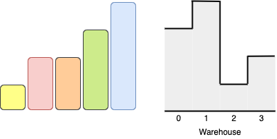
Input: boxes = [1,2,2,3,4], warehouse = [3,4,1,2]
Output: 4
Explanation:
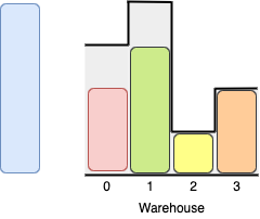
We can store the boxes in the following order:
Put the box of size 1 in room 2 from either the left or right side.
Put a box of size 2 in room 3 from the right side.
Put the box of size 3 in room 1 from the left side.
Put the other box of size 2 in room 0 from the left side.
Notice that there are other valid ways to put four boxes such as swapping the boxes of size 2 or boxes of room 0 and 1.
Example 2:
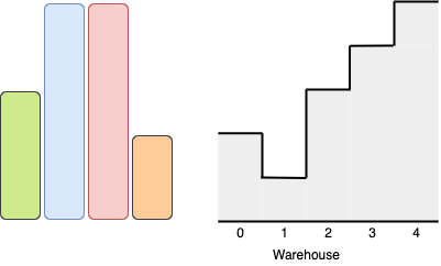
Input: boxes = [3,5,5,2], warehouse = [2,1,3,4,5]
Output: 3
Explanation:
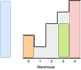
It is not possible to put the two boxes of height 5 in the warehouse since there's only one room of height >= 5.
We can put the box of size 2 in room 0 from the left side, the box of size 3 in room 3 from the right size and a box of size 5 in room 4 from the right side.
Other valid solutions are to put the box of size 3 in room 2 or to put the box of size 2 first in room 2 before putting the rest of the boxes (3 and 5)
Constraints:
n == warehouse.length1 <= boxes.length, warehouse.length <= 10^51 <= boxes[i], warehouse[i] <= 10^9
Approach 1: Two Pointer and Greedy Technique
Understanding the Core Idea
The central concept of this solution is to leverage a two-pointer technique combined with a greedy approach to maximize the number of boxes that can be placed in the warehouse. The solution exploits the flexibility of placing boxes from either end of the warehouse to optimize box placement.
Greedy Box Selection: The boxes are sorted in descending order, prioritizing larger boxes for placement first.
Two-Pointer Technique: Two pointers (left and right) are used to track available spaces at both ends of the warehouse.
Flexible Placement: The algorithm attempts to place each box at either end of the warehouse, whichever allows for placement.
Early Termination: The process stops when all warehouse rooms have been considered (pointers meet).
Code Walkthrough
Initialization: The function starts by initializing
max_numberto keep track of the number of boxes placed, and two pointersleft_indexandright_indexto represent the current available positions from the left and right ends of the warehouse, respectively.max_number = 0 left_index, right_index = 0, len(warehouse) - 1Sorting Boxes: The boxes are sorted in descending order to prioritize placing the largest boxes first.
for box in sorted(boxes, reverse=True):Placing Boxes: The function iterates through each sorted box and tries to place it either from the left or the right of the warehouse:
Left Placement: If the current box can fit in the leftmost available position (
warehouse[left_index]), it is placed there,max_numberis incremented, andleft_indexis moved to the next position.if box <= warehouse[left_index]: max_number += 1 left_index += 1Right Placement: If the current box does not fit on the left but can fit in the rightmost available position (
warehouse[right_index]), it is placed there,max_numberis incremented, andright_indexis moved to the previous position.elif box <= warehouse[right_index]: max_number += 1 right_index -= 1
Early Termination: If the two pointers meet (
left_index == right_index), the loop terminates early as no more boxes can be placed.if left_index == right_index: return max_numberResult Calculation/Return: Finally, the function returns the total number of boxes placed.
return max_number
Example
Input: boxes = [5, 4, 3, 2, 1], warehouse = [4, 3, 1, 5, 2, 3]
Step-by-Step Walkthrough:
Initialization:
max_number = 0: Initialize the count of placed boxes.left_index = 0: Set the left pointer to the first room.right_index = 5: Set the right pointer to the last room (len(warehouse) - 1).
Main Loop (Placing Boxes):
Iteration 1 (Box height: 5):
Left room height (warehouse[0]) = 4, Right room height (warehouse[5]) = 3
The box doesn't fit on either side, so it's skipped.
max_numberremains 0, indices unchanged.
Iteration 2 (Box height: 4):
Left room height (warehouse[0]) = 4, Right room height (warehouse[5]) = 3
The box fits on the left side (4 <= 4).
Place the box, increment
max_numberto 1, andleft_indexto 1.
Iteration 3 (Box height: 3):
Left room height (warehouse[1]) = 3, Right room height (warehouse[5]) = 3
The box fits on the left side (3 <= 3).
Place the box, increment
max_numberto 2, andleft_indexto 2.
Iteration 4 (Box height: 2):
Left room height (warehouse[2]) = 1, Right room height (warehouse[5]) = 3
The box doesn't fit on the left but fits on the right (2 <= 3).
Place the box, increment
max_numberto 3, and decrementright_indexto 4.
Iteration 5 (Box height: 1):
Left room height (warehouse[2]) = 1, Right room height (warehouse[4]) = 2
The box fits on the left side (1 <= 1).
Place the box, increment
max_numberto 4, andleft_indexto 3.
Loop Termination:
The loop terminates after processing all boxes.
Final state:
max_number = 4,left_index = 3,right_index = 4
Visual Aid:
Room
Box Height
Left Room Height
Right Room Height
Action
Max Number
1
5
warehouse[0] = 4
warehouse[5] = 3
Not placed
0
2
4
warehouse[0] = 4
warehouse[5] = 3
Placed on the left, increase left_index
1
3
3
warehouse[1] = 3
warehouse[5] = 3
Placed on the left, increase left_index
2
4
2
warehouse[2] = 1
warehouse[5] = 3
Placed on the right, decrease right_index
3
5
1
warehouse[2] = 1
warehouse[4] = 2
Placed on the left, increase left_index
4
Result Calculation/Final Steps:
The algorithm has placed four boxes in total.
The function returns
max_number, which is 4.
The algorithm successfully places 4 out of 5 boxes in the warehouse, optimizing the placement by considering both ends of the warehouse and prioritizing larger boxes.
Complexity Analysis
Time Complexity:
O
, where is the number of boxes. This is because: Sorting the boxes takes
time. The later iteration through the sorted boxes takes
time. The dominant factor is the sorting operation, hence
overall.
Space Complexity:
, where is the number of boxes. The space complexity is due to the built-in Tim Sort that in the worst case can use space.
In summary, this solution efficiently places the maximum number of boxes into the warehouse by sorting the boxes and using a two-pointer technique to use space from both ends, with a time complexity of
Week 4 -> 2743. Count Substrings Without Repeating Character
You are given a string s consisting only of lowercase English letters. We call a substring special if it contains no character that has occurred at least twice (in other words, it does not contain a repeating character). Your task is to count the number of special substrings. For example, in the string "pop", the substring "po" is a special substring, however, "pop" is not special (since 'p' has occurred twice).
Return the number of special substrings.
A substring is a contiguous sequence of characters within a string. For example, "abc" is a substring of "abcd", but "acd" is not.
Example 1:
Input: s = "abcd"
Output: 10
Explanation: Since each character occurs once, every substring is a special substring. We have 4 substrings of length one, 3 of length two, 2 of length three, and 1 substring of length four. So overall, there are 4 + 3 + 2 + 1 = 10 special substrings.
Example 2:
Input: s = "ooo"
Output: 3
Explanation: Any substring with a length of at least two contains a repeating character. So we have to count the number of substrings of length one, which is 3.
Example 3:
Input: s = "abab"
Output: 7
Explanation: Special substrings are as follows (sorted by their start positions):
Special substrings of length 1: "a", "b", "a", "b"
Special substrings of length 2: "ab", "ba", "ab"
And it can be shown that there are no special substrings with a length of at least three. So the answer would be 4 + 3 = 7.
Constraints:
1 <= s.length <= 10^5sconsists of lowercase English letters
Approach 1: Sliding Window with Set
Understanding the Core Idea
The central concept of this solution is to leverage a sliding window technique combined with a set data structure to efficiently count special substrings. This approach takes advantage of the problem's nature by counting non-special substrings and subtracting them from the total possible substrings.
Sliding Window: The solution uses a variable-size sliding window to keep track of the current substring being considered.
Set for Uniqueness: A set is used to maintain the unique characters in the current window, allowing for constant-time lookups.
Subtraction Strategy: Instead of directly counting special substrings, the algorithm starts with the total number of all possible substrings and subtracts the count of non-special substrings.
Code Walkthrough
Initialization:
window_chars = set() left_index = 0 n = len(s) potential_special_substrings = n * (n + 1) // 2The code initializes an empty set
window_charsto store unique characters,left_indexto mark the start of the window, and calculates the total number of possible substrings. The total number of substrings works with that formula because for each character at position i, there aren - isubstrings that end at that position; since we also count substrings of length 1, we add the total number o substrings of length 1 to the total to get the formula. Iterating Through Characters:
for current_char in s:The main loop iterates through each character in the input string.
Window Adjustment:
while current_char in window_chars: window_chars.remove(s[left_index]) left_index += 1If the current character is already in the window, the window is shrunk from the left until the current character becomes unique in the window.
Counting Non-Special Substrings:
potential_special_substrings -= left_indexThe number of non-special substrings ending at the current position is equal to
left_index. This is subtracted from the total count.Updating Window:
window_chars.add(current_char)The current character is added to the set of window characters.
Result Calculation/Return:
return potential_special_substringsAfter processing all characters, the remaining count in
potential_special_substringsrepresents the number of special substrings.
Example
Input:
Step-by-Step Walkthrough:
Initialization:
Set
window_chars = set()to keep track of unique characters in the current window.Set
left_index = 0to mark the start of the current window.Set
n = len(s) = 4(length of the input string).Calculate
potential_special_substrings = n * (n + 1) // 2 = 4 * (4 + 1) // 2 = 10. This represents the total number of all possible substrings.
Main Loop (Iterate through each character in the string):
Iteration 1: Character 'a' at index 0
Current state:
window_chars = set(),left_index = 0Check if 'a' is in
window_chars: It's not, so we don't need to shrink the window.Calculate non-special substrings ending at this position:
left_index = 0Update
potential_special_substrings = 10 - 0 = 10Add 'a' to
window_chars:window_chars = {'a'}
Iteration 2: Character 'b' at index 1
Current state:
window_chars = {'a'},left_index = 0Check if 'b' is in
window_chars: It's not, so we don't need to shrink the window.Calculate non-special substrings ending at this position:
left_index = 0Update
potential_special_substrings = 10 - 0 = 10Add 'b' to
window_chars:window_chars = {'a', 'b'}
Iteration 3: Character 'a' at index 2
Current state:
window_chars = {'a', 'b'},left_index = 0Check if 'a' is in
window_chars: It is, so we need to shrink the window.Remove 's[left_index]' ('a') from
window_charsIncrement
left_indexto 1
Calculate non-special substrings ending at this position:
left_index = 1Update
potential_special_substrings = 10 - 1 = 9Add 'a' to
window_chars:window_chars = {'a', 'b'}
Iteration 4: Character 'b' at index 3
Current state:
window_chars = {'a', 'b'},left_index = 1Check if 'b' is in
window_chars: It is, so we need to shrink the window.Remove 's[left_index]' ('b') from
window_charsIncrement
left_indexto 2
Calculate non-special substrings ending at this position:
left_index = 2Update
potential_special_substrings = 9 - 2 = 7Add 'b' to
window_chars:window_chars = {'a', 'b'}
Loop Termination:
The loop ends after processing all characters in the string.
Final state:
window_chars = {'a', 'b'},left_index = 2,potential_special_substrings = 7
Visual Aid:
Here's a table summarizing each iteration:
Position
Character
Left Index
Window Chars
Non-special Count
Potential Special
1
a
0
['a']
0
10
2
b
0
['a', 'b']
0
10
3
a
1
['a', 'b']
1
9
4
b
2
['a', 'b']
2
7
Result Calculation:
The algorithm starts with the total number of all possible substrings (10) and subtracts the count of non-special substrings at each step.
The final value of
potential_special_substrings(7) represents the count of special substrings.Therefore, the function returns 7 as the final count of special substrings in "abab".
The special substrings are: "a", "b", "a", "b", "ab", "ba", "ab".
Approach 2: Sliding Window with Last Occurrence Array
Understanding the Core Idea
The central concept of this solution is to leverage a sliding window technique combined with an array to track the last occurrence of each character. This approach efficiently counts special substrings by maintaining the most recent valid window for each character encountered.
Sliding Window: The solution uses a variable-size sliding window to keep track of the current substring being considered.
Last Occurrence Array: An array is used to store the index of the last occurrence of each character, allowing for constant-time lookups and updates.
Counting Strategy: The algorithm counts special substrings directly by calculating the number of valid substrings ending at each character.
Code Walkthrough
Initialization:
special_substrings_count = 0 last_occurrence = [-1] * 26 start_index = 0The code initializes the count of special substrings, an array to store the last occurrence of each character (initialized to -1), and the start index of the current window.
Iterating Through Characters:
for current_index, char in enumerate(s):The main loop iterates through each character in the input string, keeping track of both the character and its index.
Character Index Calculation:
char_index = ord(char) - ord('a')Calculates the index for the current character in the
last_occurrencearray.Window Adjustment:
if last_occurrence[char_index] >= start_index: start_index = last_occurrence[char_index] + 1If the current character has appeared before within the current window, the window's start is moved to just after the last occurrence of this character.
Counting Special Substrings:
special_substrings_count += current_index - start_index + 1Counts the number of special substrings ending at the current character. This is equal to the size of the current window.
Updating Last Occurrence:
last_occurrence[char_index] = current_indexUpdates the last occurrence index for the current character.
Result Calculation/Return:
return special_substrings_countAfter processing all characters, the total count of special substrings is returned.
Complexity Analysis
Time Complexity:
, where is the length of the input string. This is because the algorithm iterates through each character in the string exactly once, performing constant-time operations at each step.
Space Complexity:
, because the last_occurrencearray has a fixed size of 26 elements (one for each lowercase English letter), regardless of the input string's length. While this could be written aswhere is the size of the alphabet, since is fixed at 26, it's considered constant space.
Example
Input:
Step-by-Step Walkthrough:
Initialization:
Set
special_substrings_count = 0to keep track of the number of special substrings.Initialize
last_occurrence = [-1] * 26, an array to store the last occurrence index of each lowercase letter.Set
start_index = 0to mark the start of the current valid window.Set
n = len(s) = 4(length of the input string).
Main Loop (Iterate through each character in the string):
Iteration 1: Character 'a' at index 0
Calculate
char_index = ord('a') - ord('a') = 0Check if 'a' occurred within the current window:
last_occurrence[0] = -1, which is less thanstart_index = 0, so no adjustment is needed.
Count special substrings:
New special substrings =
current_index - start_index + 1 = 0 - 0 + 1 = 1Update
special_substrings_count = 0 + 1 = 1
Update
last_occurrence[0] = 0
Iteration 2: Character 'b' at index 1
Calculate
char_index = ord('b') - ord('a') = 1Check if 'b' occurred within the current window:
last_occurrence[1] = -1, which is less thanstart_index = 0, so no adjustment is needed.
Count special substrings:
New special substrings =
current_index - start_index + 1 = 1 - 0 + 1 = 2Update
special_substrings_count = 1 + 2 = 3
Update
last_occurrence[1] = 1
Iteration 3: Character 'a' at index 2
Calculate
char_index = ord('a') - ord('a') = 0Check if 'a' occurred within the current window:
last_occurrence[0] = 0, which is not less thanstart_index = 0Update
start_index = last_occurrence[0] + 1 = 0 + 1 = 1
Count special substrings:
New special substrings =
current_index - start_index + 1 = 2 - 1 + 1 = 2Update
special_substrings_count = 3 + 2 = 5
Update
last_occurrence[0] = 2
Iteration 4: Character 'b' at index 3
Calculate
char_index = ord('b') - ord('a') = 1Check if 'b' occurred within the current window:
last_occurrence[1] = 1, which is not less thanstart_index = 1Update
start_index = last_occurrence[1] + 1 = 1 + 1 = 2
Count special substrings:
New special substrings =
current_index - start_index + 1 = 3 - 2 + 1 = 2Update
special_substrings_count = 5 + 2 = 7
Update
last_occurrence[1] = 3
Loop Termination:
The loop ends after processing all characters in the string.
Final state:
special_substrings_count = 7,start_index = 2,last_occurrence = [2, 3, -1, -1, -1, ...]
Visual Aid:
Here's a table summarizing each iteration:
Position
Character
Char Index
Start Index
New Special
Total Special
Last Occurrence
1
a
0
0
1
1
[0, -1, -1, -1, -1] + ["..."]
2
b
1
0
2
3
[0, 1, -1, -1, -1] + ["..."]
3
a
0
1
2
5
[2, 1, -1, -1, -1] + ["..."]
4
b
1
2
2
7
[2, 3, -1, -1, -1] + ["..."]
Result Calculation:
The algorithm directly calculates the count of special substrings at each step.
For each character, it counts the number of special substrings ending at that character, which is the length of the current valid window.
The
special_substrings_countis updated cumulatively, so the final value (7) represents the total count of special substrings in "abab".
The special substrings are: "a", "b", "a", "b", "ab", "ba", "ab".
Week 5 -> 776. Split BST
Given the root of a binary search tree (BST) and an integer target, split the tree into two subtrees where the first subtree has nodes that are all smaller or equal to the target value, while the second subtree has all nodes that are greater than the target value. It is not necessarily the case that the tree contains a node with the value target.
Additionally, most of the structure of the original tree should remain. Formally, for any child c with parent p in the original tree, if they are both in the same subtree after the split, then node c should still have the parent p.
Return an array of the two roots of the two subtrees in order.
Example 1:

Input: root = [4,2,6,1,3,5,7], target = 2
Output: [[2,1],[4,3,6,null,null,5,7]]
Example 2:
Input: root = [1], target = 1
Output: [[1],[]]
Constraints:
The number of nodes in the tree is in the range
[1, 50].0 <= Node.val, target <= 1000
Approach 1: Iterative BST Traversal and Reconstruction
Understanding the Core Idea
The central concept of this solution is to leverage an iterative traversal of the Binary Search Tree (BST) to split it into two subtrees based on a target value. This approach efficiently maintains the BST structure while separating nodes into two categories: those with values less than or equal to the target, and those with values greater than the target.
Iterative Traversal: The solution uses an iterative method with a stack to traverse the BST, avoiding the potential stack overflow issues of a recursive approach for very deep trees.
In-place Reconstruction: Instead of creating new nodes, the algorithm reconstructs the two subtrees by modifying the existing tree structure, which is memory-efficient.
Path Tracking: A stack is used to keep track of the traversal path, which is crucial for the reconstruction phase.
Code Walkthrough
Initialization:
smaller_equal_subtree, greater_subtree = None, None path_stack = []We initialize two variables to store the roots of our resulting subtrees and an empty stack to keep track of our traversal path.
Downward Traversal:
current = root while current: path_stack.append(current) if current.val <= target: current = current.right else: current = current.leftThis loop traverses down the tree, always choosing the right child if the current node's value is less than or equal to the target, and the left child otherwise. Each visited node is added to the
path_stack. This ensures we only traverse one path of the tree, which is key to the algorithm's efficiency.Upward Reconstruction:
while path_stack: node = path_stack.pop() if node.val <= target: node.right = smaller_equal_subtree smaller_equal_subtree = node else: node.left = greater_subtree greater_subtree = nodeWe now pop nodes from the stack (which reverses our traversal order) and reconstruct our two subtrees. If a node's value is less than or equal to the target, we make it the new root of the
smaller_equal_subtreeand set its right child to the previoussmaller_equal_subtree. If it's greater, we do the same for thegreater_subtree, but with the left child. This preserves the BST property in both resulting trees.Result Return:
return [smaller_equal_subtree, greater_subtree]Finally, we return a list containing the roots of our two reconstructed subtrees.
Complexity Analysis
Time Complexity:
, where is the height of the tree. This is because we traverse down one path of the tree and then back up. In the worst case (a completely unbalanced tree), this becomes , where is the number of nodes.
Space Complexity:
, where is the height of the tree. This is due to the stack used to store the path, which in the worst case (a completely unbalanced tree) stores all nodes, resulting in space complexity.
The space complexity is generally better than a recursive solution, especially for very deep trees, as it avoids the overhead of recursive function calls on the system stack.
Example
Input:
A visual representation of the input BST:
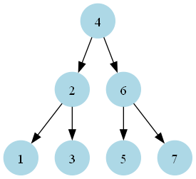
Step-by-Step Walkthrough:
Initialization:
Initialize
smaller_equal_subtree = Noneandgreater_subtree = None.Create an empty list
path_stack = []to store the traversal path.Set
current = root(the node with value 4).
Main Loop (Traversing down the tree):
Iteration 1:
current.val(4) >target(2)Append
current(4) topath_stackMove to the left child:
current = current.left(node with value 2)path_stackis now [4]
Iteration 2:
current.val(2) <=target(2)Append
current(2) topath_stackMove to the right child:
current = current.right(node with value 3)path_stackis now [4, 2]
Iteration 3:
current.val(3) >target(2)Append
current(3) topath_stackMove to the left child:
current = current.left(which is None)path_stackis now [4, 2, 3]
Loop Termination:
The loop ends when
currentbecomes NoneAt this point,
path_stackcontains [4, 2, 3]
Visual Aid: Traversal Summary
Iteration
Current Node
Path Stack
Direction
1
4
[4]
Left
2
2
[4, 2]
Right
3
3
[4, 2, 3]
Left
Result Calculation/Final Steps:
Now we reconstruct the subtrees by popping nodes from
path_stack:Pop 3:
3 > 2, so set
node.left = greater_subtree(None)Update
greater_subtree = node(3)Visual representation of the greater subtree:

Pop 2:
2 <= 2, so set
node.right = smaller_equal_subtree(None)Update
smaller_equal_subtree = node(2)Visual representation of the smaller or equal subtree:

Pop 4:
4 > 2, so set
node.left = greater_subtree(3)Update
greater_subtree = node(4)Visual representation of the greater subtree:
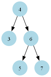
The loop ends as
path_stackis empty
Final state:
smaller_equal_subtree: Root 2, with left child 1greater_subtree: Root 4, with left child 3 and right subtree unchanged (6, 5, 7)
The function returns [smaller_equal_subtree, greater_subtree], which represents the two split subtrees based on target value 2.
Approach 2: Recursive BST Traversal and Reconstruction
Understanding the Core Idea
The central concept of this solution is to leverage a recursive traversal of the Binary Search Tree (BST) to split it into two subtrees based on a target value. This approach efficiently maintains the BST structure while separating nodes into two categories: those with values less than or equal to the target, and those with values greater than the target.
Recursive Traversal: The solution uses a recursive method to traverse the BST, which aligns closely with the tree's inherent recursive structure.
In-place Reconstruction: Instead of creating new nodes, the algorithm reconstructs the two subtrees by modifying the existing tree structure, which is memory-efficient.
Divide and Conquer: The problem is solved by breaking it down into smaller subproblems (subtrees) and combining their results.
Code Walkthrough
Helper Function Definition:
def split_tree(node: Optional[TreeNode]) -> List[Optional[TreeNode]]:A helper function is defined to perform the recursive splitting. It returns a list of two subtrees: one with nodes less than or equal to the target, and one with nodes greater than the target.
Base Case:
if not node: return [None, None]If the current node is None, we've reached a leaf, so we return two None values representing empty subtrees.
Recursive Case for Nodes Less Than or Equal to Target:
if node.val <= target: smaller_equal_subtree, greater_subtree = split_tree(node.right) node.right = smaller_equal_subtree return [node, greater_subtree]If the current node's value is less than or equal to the target, we recursively split its right subtree. We then update the current node's right child to be the smaller/equal part of the split right subtree. We return the current node as the root of the smaller/equal subtree along with the greater part of the split right subtree.
Recursive Case for Nodes Greater Than Target:
else: smaller_equal_subtree, greater_subtree = split_tree(node.left) node.left = greater_subtree return [smaller_equal_subtree, node]If the current node's value is greater than the target, we recursively split its left subtree. We then update the current node's left child to be the greater part of the split left subtree. We return the smaller/equal part of the split left subtree along with the current node as the root of the greater subtree.
Main Function Call:
return split_tree(root)The main function simply calls the helper function with the root of the tree and returns its result.
Complexity Analysis
Time Complexity:
, where is the height of the tree. This is because we traverse down one path of the tree, making a decision at each node whether to go left or right based on the target value. In the worst case (a completely unbalanced tree), this becomes , where is the number of nodes.
Space Complexity:
, where is the height of the tree. This is due to the recursive call stack, which in the worst case (a completely unbalanced tree) can go as deep as the number of nodes, resulting in space complexity.
The space complexity could be a concern for very deep trees, as it might lead to stack overflow errors. However, for balanced trees, the space complexity remains logarithmic in the number of nodes.
Example
Input:
A visual representation of the input BST:

Step-by-Step Walkthrough:
Initialization:
The function
splitBST2is called withroot(node with value 4) andtarget = 2.It immediately calls the helper function
split_tree(root).
Main Recursive Process:
Recursive call at depth 0:
Current node: 4
4 > 2, so we recurse on the left child
Recursive call at depth 1:
Current node: 2
2 <= 2, so we recurse on the right child
Recursive call at depth 2:
Current node: 3
3 > 2, so we recurse on the left child
Recursive call at depth 3:
Current node: None
Base case reached, return
[None, None]
Unwinding the Recursion:
Back to depth 2 (node 3):
Received
[None, None]from left childSet
node.left = None(greater subtree)Return
[None, 3](smaller_equal_subtree, node)Visual representation of the smaller or equal subtree:

Back to depth 1 (node 2):
Received
[None, 3]from right childSet
node.right = None(smaller_equal_subtree)Return
[2, 3](node, greater_subtree)Visual representation of the greater subtree:

Back to depth 0 (node 4):
Received
[2, 3]from left childSet
node.left = 3(greater subtree)Return
[2, 4](smaller_equal_subtree, node)Visual representation of the updated greater subtree:

Visual Aid: Reconstruction Summary
Depth
Processed Node
Subtree Added To
Smaller/Equal Subtree Root
Greater Subtree Root
2
3
greater
3
1
2
smaller_equal
2
3
0
4
greater
2
4
Result Calculation/Final Steps:
The recursion completes, and
split_tree(root)returns[2, 4].This result is directly returned by
splitBST2.
Final state:
smaller_equal_subtree: Root 2, with left child 1 and right child Nonegreater_subtree: Root 4, with left child 3 and right subtree unchanged (6, 5, 7)
The function returns [smaller_equal_subtree, greater_subtree], which represents the two split subtrees based on target value 2. The recursive approach efficiently splits the tree in a single pass, leveraging the BST property to make decisions at each node.
Approach 3: Iterative In-Place BST Reconstruction
Understanding the Core Idea
The central concept of this solution is to leverage an iterative traversal of the Binary Search Tree (BST) to split it into two subtrees based on a target value. This approach reconstructs the two subtrees in-place using pointer manipulation, without using additional data structures like stacks or recursion.
Iterative Traversal: The solution uses an iterative method to traverse the BST, avoiding potential stack overflow issues associated with recursive approaches for very deep trees.
In-Place Reconstruction: The algorithm reconstructs the two subtrees by modifying the existing tree structure through pointer manipulation, which is memory-efficient.
Dummy Nodes: The use of dummy nodes simplifies the process of building the new subtrees, eliminating the need for special cases when adding the first node to each subtree.
Code Walkthrough
Initialization:
dummy_smaller_equal = TreeNode() dummy_greater = TreeNode() current_smaller_equal = dummy_smaller_equal current_greater = dummy_greater current_node = rootWe initialize dummy nodes for both subtrees and set up pointers to the current positions in each subtree.
current_nodeis initialized to the root of the original tree.Main Traversal Loop:
while current_node is not None:This loop continues until we've processed all nodes in the original tree.
Processing Nodes Less Than or Equal to Target:
if current_node.val <= target: current_smaller_equal.right = current_node current_smaller_equal = current_node next_node = current_node.right current_smaller_equal.right = None # Cut off right subtreeIf the current node's value is less than or equal to the target, we add it to the smaller/equal subtree. We update pointers, save the right child as the next node to process, and cut off the right subtree to maintain the BST property.
Processing Nodes Greater Than Target:
else: current_greater.left = current_node current_greater = current_node next_node = current_node.left current_greater.left = None # Cut off left subtreeIf the current node's value is greater than the target, we add it to the greater subtree. We update pointers, save the left child as the next node to process, and cut off the left subtree to maintain the BST property.
Moving to the Next Node:
current_node = next_nodeWe move to the next node to process, which was saved earlier as either the left or right child of the current node.
Result Preparation and Return:
smaller_equal_subtree = dummy_smaller_equal.right greater_subtree = dummy_greater.left return [smaller_equal_subtree, greater_subtree]We extract the actual roots of our new subtrees (skipping the dummy nodes) and return them as a list.
Complexity Analysis
Time Complexity:
, where is the height of the tree. This is because the algorithm traverses a single path from the root to a leaf, making a decision at each node whether to go left or right based on the target value. In the best and average cases (balanced BST), this results in
time complexity, where is the number of nodes in the tree. In the worst case (completely unbalanced BST), this could become
.
Space Complexity:
, as it uses only a constant amount of extra space regardless of input size. The algorithm uses a fixed number of pointers and doesn't rely on any additional data structures that grow with the input size.
This approach is particularly helpful for large trees or in memory-constrained environments, as it avoids the risk of stack overflow and uses minimal extra memory.
Example
Input:
A visual representation of the input BST:

Step-by-Step Walkthrough:
Initialization:
Create
dummy_smaller_equalanddummy_greateras dummy TreeNodes.Set
current_smaller_equal = dummy_smaller_equalSet
current_greater = dummy_greaterSet
current_node = root(node with value 4)
Main Loop:
Iteration 1:
current_node.val(4) >target(2)Add to greater subtree:
Set
current_greater.left = current_node(4)Update
current_greater = current_node(4)
Set
next_node = current_node.left(2)Cut off left subtree:
current_greater.left = NoneUpdate
current_node = next_node(2)Visual representation of the greater subtree with dummy node:
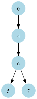
Iteration 2:
current_node.val(2) <=target(2)Add to smaller_equal subtree:
Set
current_smaller_equal.right = current_node(2)Update
current_smaller_equal = current_node(2)
Set
next_node = current_node.right(3)Cut off right subtree:
current_smaller_equal.right = NoneUpdate
current_node = next_node(3)Visual representation of the smaller or equal subtree with dummy node:

Iteration 3:
current_node.val(3) >target(2)Add to greater subtree:
Set
current_greater.left = current_node(3)Update
current_greater = current_node(3)
Set
next_node = current_node.left(None)Cut off left subtree:
current_greater.left = NoneUpdate
current_node = next_node(None)Visual representation of the greater subtree with dummy node:
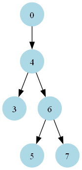
Loop Termination:
The loop ends when
current_nodebecomes None
Visual Aid: Iteration Summary
Iteration
Current Smaller/Equal
Current Greater
Next Node
1
4
2
2
2
4
3
3
2
3
Result Calculation/Final Steps:
Set
smaller_equal_subtree = dummy_smaller_equal.right(2)Set
greater_subtree = dummy_greater.left(4)
Final state:
smaller_equal_subtree: Root 2, with left child 1 and right child Nonegreater_subtree: Root 4, with left child 3 and right subtree unchanged (6, 5, 7)
The final visual representation of the two subtrees:
Smaller or Equal Subtree:

Greater Subtree:

The function returns [smaller_equal_subtree, greater_subtree], which represents the two split subtrees based on target value 2. This iterative approach efficiently splits the tree in a single pass without using recursion or additional stack space, making it memory-efficient and suitable for very deep trees.