July 2024, Week 3: July 15th - July 21st
July 15 -> 2196. Create Binary Tree From Descriptions
You are given a 2D integer array descriptions where descriptions[i] = [parent_i, child_i, isLeft_i] indicates that parent_i is the parent of child_i in a binary tree of unique values. Furthermore,
If
isLeft_i == 1, thenchild_iis the left child ofparent_i.If
isLeft_i == 0, thenchild_iis the right child ofparent_i.
Construct the binary tree described by descriptions and return its root.
The test cases will be generated such that the binary tree is valid.
Example 1:
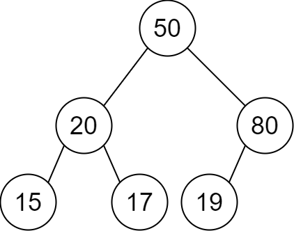
Input:
descriptions = [[20,15,1],[20,17,0],[50,20,1],[50,80,0],[80,19,1]]Output:
[50,20,80,15,17,19]Explanation: The root node is the node with value 50 since it has no parent. The resulting binary tree is shown in the diagram.
Example 2:
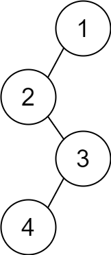
Input:
descriptions = [[1,2,1],[2,3,0],[3,4,1]]Output:
[1,2,null,null,3,4]Explanation: The root node is the node with value 1 since it has no parent. The resulting binary tree is shown in the diagram.
Constraints:
1 <= descriptions.length <= 10^4descriptions[i].length == 31 <= parent_i, child_i <= 10^50 <= isLeft_i <= 1The binary tree described by
descriptionsis valid.
Approach 1: Hash Map and Single-Pass Construction
Understanding the Core Idea
The central concept of this solution is to leverage a hash map (dictionary) to efficiently construct the binary tree in a single pass through the descriptions. This approach exploits the property that each node in a binary tree has a unique value, allowing us to use these values as keys in our hash map.
Node Storage: Each unique node is stored in a hash map, allowing
access when connecting parent-child relationships. Root Identification: The root is identified as the only parent node that doesn't appear as a child in any description.
Tree Construction: The tree is built incrementally by processing each description and connecting nodes based on the given parent-child relationships.
Code Walkthrough
Initialization:
# Create a map of child values to their corresponding nodes node_map = {child: BinaryTreeNode(child) for _, child, _ in descriptions}This line creates a dictionary
node_mapwhere each key is a child value from the descriptions, and the corresponding value is a newBinaryTreeNodewith that value. This initializes all nodes that appear as children in the descriptions.Root Initialization and Tree Construction:
root = None for parent_value, child_value, is_left_child in descriptions: if parent_value not in node_map: # Create root node (the only parent value not present as a child) root = node_map[parent_value] = BinaryTreeNode(parent_value)This loop iterates through each description. If a parent value is encountered that's not in the
node_map, it means this node hasn't been seen as a child before, so it must be the root. We create this node and assign it to bothrootandnode_map[parent_value].Child Assignment:
# Assign child node to appropriate side of parent if is_left_child: node_map[parent_value].left = node_map[child_value] else: node_map[parent_value].right = node_map[child_value]For each description, we assign the child node to either the left or right of the parent node based on the
is_left_childvalue. Both parent and child nodes are accessed from thenode_mapintime. Result Return:
return rootAfter processing all descriptions, we return the root node of the constructed binary tree.
Complexity Analysis
Time Complexity:
, where is the number of descriptions (which is equal to the number of edges in the tree). We iterate through the descriptions once to create the node_map, and then again to construct the tree. Both operations are, resulting in a total time complexity of .
Space Complexity:
, where is the number of descriptions. The node_mapstores one entry for each unique node in the tree. In the worst case, this could be up tonodes ( child nodes plus one root node that only appears as a parent). Therefore, the space complexity is .
Example
Input:
Step-by-Step Walkthrough:
Initialization:
The function starts by creating a
node_mapdictionary. This map uses child values as keys andBinaryTreeNodeobjects as values.Initial
node_map:node_map = { 58: BinaryTreeNode(58), 39: BinaryTreeNode(39), 45: BinaryTreeNode(45), 43: BinaryTreeNode(43), 41: BinaryTreeNode(41), 52: BinaryTreeNode(52) }rootis initialized asNone.
Main Algorithm Process:
Iteration 1:
Processing
[52, 58, 0]52is innode_map, so no new node is created.58is assigned as the right child of52becauseis_left_childis0.Current tree:
52 -> 58 (right)
Iteration 2:
Processing
[41, 39, 1]41is innode_map, so no new node is created.39is assigned as the left child of41becauseis_left_childis1.Current tree:
52 -> 58 (right),41 -> 39 (left)
Iteration 3:
Processing
[52, 45, 1]52already exists innode_map.45is assigned as the left child of52(is_left_childis1).Current tree:
52 -> 58 (right), 45 (left),41 -> 39 (left)
Iteration 4:
Processing
[41, 43, 0]41already exists innode_map.43is assigned as the right child of41(is_left_childis0).Current tree:
52 -> 58 (right), 45 (left),41 -> 39 (left), 43 (right)
Iteration 5:
Processing
[45, 41, 1]45already exists innode_map.41is assigned as the left child of45(is_left_childis1).Current tree:
52 -> 58 (right), 45 (left),45 -> 41 (left),41 -> 39 (left), 43 (right)
Iteration 6:
Processing
[60, 52, 1]60is not innode_map, so a newBinaryTreeNode(60)is created and set asrootbecause it is the only parent node not present as a child.52is assigned as the left child of60.Final tree:
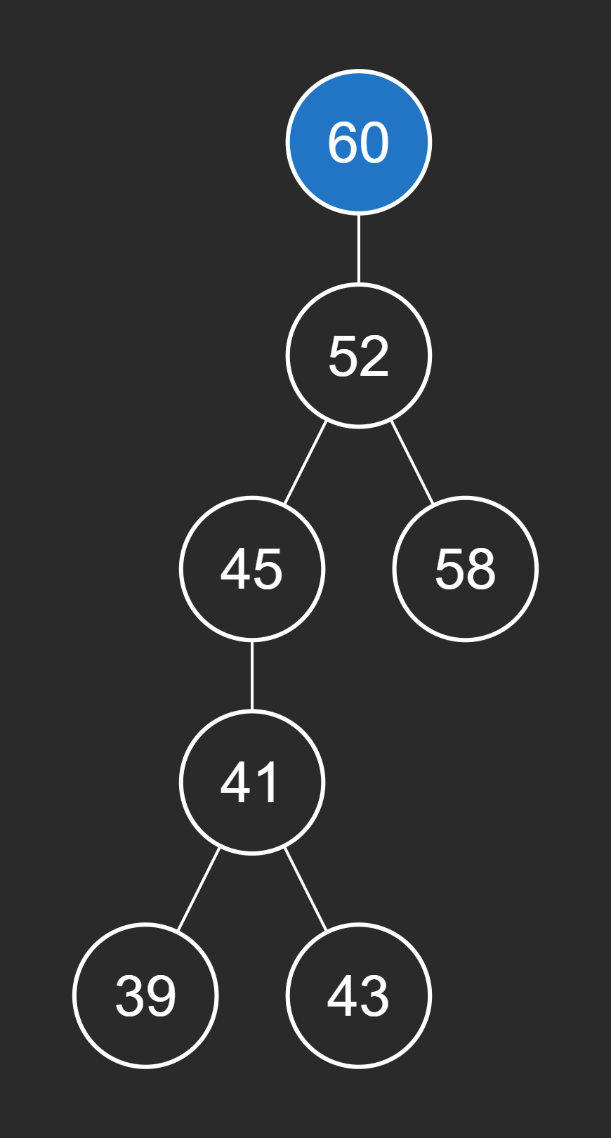
60 -> 52 (left),52 -> 58 (right), 45 (left),45 -> 41 (left),41 -> 39 (left), 43 (right)
Loop Termination:
The loop terminates after processing all descriptions in the input list.
The final state of the tree is complete, with
60as the root node.
Visual Aid: Here's a summary table of the iterations:
Iteration
Parent
Child
Child Position
Parent Node Status
1
52
58
Right
Existed
2
41
39
Left
Existed
3
52
45
Left
Existed
4
41
43
Right
Existed
5
45
41
Left
Existed
6
60
52
Left
Created
Result Calculation/Final Steps:
After processing all descriptions, the function has constructed the entire binary tree.
The
rootvariable holds the reference to the root node of the tree, which is60.The function returns this
rootnode, representing the entire constructed binary tree.
The final tree structure looks like this:
July 16 -> 2096. Step-By-Step Directions From a Binary Tree Node to Another
You are given the root of a binary tree with n nodes. Each node is uniquely assigned a value from 1 to n. You are also given an integer startValue representing the value of the start node s, and a different integer destValue representing the value of the destination node t.
Find the shortest path starting from node s and ending at node t. Generate step-by-step directions of such path as a string consisting of only the uppercase letters 'L', 'R', and 'U'. Each letter indicates a specific direction:
'L'means to go from a node to its left child node.'R'means to go from a node to its right child node.'U'means to go from a node to its parent node.
Return the step-by-step directions of the shortest path from node s to node t.
Example 1:
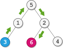
Input:
root = [5,1,2,3,null,6,4], startValue = 3, destValue = 6Output:
"UURL"Explanation: The shortest path is: 3 → 1 → 5 → 2 → 6.
Example 2:

Input:
root = [2,1], startValue = 2, destValue = 1Output:
"L"Explanation: The shortest path is: 2 → 1.
Constraints:
The number of nodes in the tree is
n.2 <= n <= 10^51 <= Node.val <= nAll the values in the tree are unique.
1 <= startValue, destValue <= nstartValue != destValue
Approach 1: Lowest Common Ancestor (LCA) with Path Reconstruction
Understanding the Core Idea
The central concept of this solution is to leverage the Lowest Common Ancestor (LCA) algorithm to find the meeting point of the paths from the start node to the destination node. This approach effectively breaks down the problem into three main steps: finding the LCA, constructing paths from the LCA to both the start and destination nodes, and then combining these paths to form the final result.
Lowest Common Ancestor (LCA): The solution first identifies the LCA of the start and destination nodes. This is the deepest node in the tree that is an ancestor of both nodes.
Path Construction: Once the LCA is found, the algorithm constructs two separate paths: one from the LCA to the start node, and another from the LCA to the destination node.
Path Combination: The final step involves combining these paths. The path to the start node is converted to a series of 'U' moves (to go up to the LCA), while the path to the destination is kept as is (to go down from the LCA).
Code Walkthrough
Defining Helper Functions:
def findCommonAncestor(node: BinaryTreeNode) -> Optional[BinaryTreeNode]: # ... (function body) def findPath(current_node: BinaryTreeNode, target_value: int, path: List[str]) -> bool: # ... (function body)These helper functions are defined within the main function to encapsulate specific tasks.
findCommonAncestoris responsible for locating the Lowest Common Ancestor (LCA) of the start and destination nodes, whilefindPathconstructs the path from a given node to a target node.Finding the Lowest Common Ancestor:
def findCommonAncestor(node: BinaryTreeNode) -> Optional[BinaryTreeNode]: # Base case: if node is None or is one of the target nodes if node is None or node.val == start_value or node.val == dest_value: return node # Recurse on left and right subtrees left_result = findCommonAncestor(node.left) right_result = findCommonAncestor(node.right) # If both subtrees return a node, this is the LCA if left_result and right_result: return node # Otherwise, return the non-None result (if any) return left_result or right_resultThis function uses a recursive approach to find the LCA. It traverses the tree, returning the node itself if it's
Noneor matches either the start or destination value. If both left and right subtrees return a non-Nonevalue, the current node is the LCA. Otherwise, it propagates the non-Noneresult upwards.Constructing Paths:
def findPath(current_node: BinaryTreeNode, target_value: int, path: List[str]) -> bool: # Recursively find the path to target node, # appending directions to 'path' if current_node.val == target_value: return True if current_node.left: path.append('L') if findPath(current_node.left, target_value, path): return True path.pop() if current_node.right: path.append('R') if findPath(current_node.right, target_value, path): return True path.pop() return FalseThis function uses depth-first search to find the path from a given node to the target node. It appends 'L' or 'R' to the
pathlist as it traverses left or right. If the target is found, it returnsTrue, propagating the success upwards. If a path doesn't lead to the target, it backtracks by removing the last direction (path.pop()).Identifying the LCA and Finding Paths:
lowest_common_ancestor = findCommonAncestor(root) path_to_start = [] path_to_dest = [] findPath(lowest_common_ancestor, start_value, path_to_start) findPath(lowest_common_ancestor, dest_value, path_to_dest)Here, we first find the LCA of the start and destination nodes. Then, we construct two paths: one from the LCA to the start node and another from the LCA to the destination node. This approach minimizes unnecessary traversals by starting from the LCA rather than the root for both paths.
Constructing the Final Path:
# Construct the final path: 'U's to go up to LCA, initial_path = 'U' * len(path_to_start) # then path down to destination final_path = ''.join(path_to_dest) return initial_path + final_pathThe final path is constructed in two parts:
initial_path: A string of 'U's with length equal to the path from LCA to start node. This represents the upward movement from the start node to the LCA.final_path: The path from LCA to the destination node, converted from a list of directions to a string.
These two parts are concatenated to form the complete path from start to destination via the LCA.
Complexity Analysis
Time Complexity:
, where is the number of nodes in the binary tree. The time complexity is linear because in the worst case, we may need to visit each node once during the LCA search. The later path constructions from the LCA to the start and destination nodes are also linear in the height of the tree, which is at most in a skewed tree.
Space Complexity:
, where is the height of the binary tree. The space complexity is determined by the maximum depth of the recursion stack during the DFS traversals. In the worst case of a skewed tree, this could be , but for a balanced tree, it would be . Additionally, we store the paths to the start and destination nodes, but these are also bounded by the height of the tree.
Example
Input:
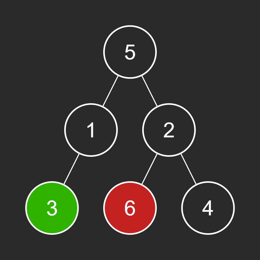
A visual representation of the binary tree with the green node representing the start node (3) and the red node representing the destination node (6) is shown below:
Step-by-Step Walkthrough:
Initialization:
The function is called with
root(a binary tree with the structure shown in the input),start_value = 3, anddest_value = 6.Two helper functions are defined within
getDirections1:findCommonAncestorandfindPath.
Finding Lowest Common Ancestor (LCA):
The
findCommonAncestorfunction is called with the root node (value 5).Iteration 1 (node 5):
Recursively calls
findCommonAncestoron left child (1) and right child (2).
Iteration 2 (node 1):
Recursively calls
findCommonAncestoron left child (3).
Iteration 3 (node 3):
Matches
start_value, returns node 3.
Iteration 4 (node 2):
Recursively calls
findCommonAncestoron left child (6).
Iteration 5 (node 6):
Matches
dest_value, returns node 6.
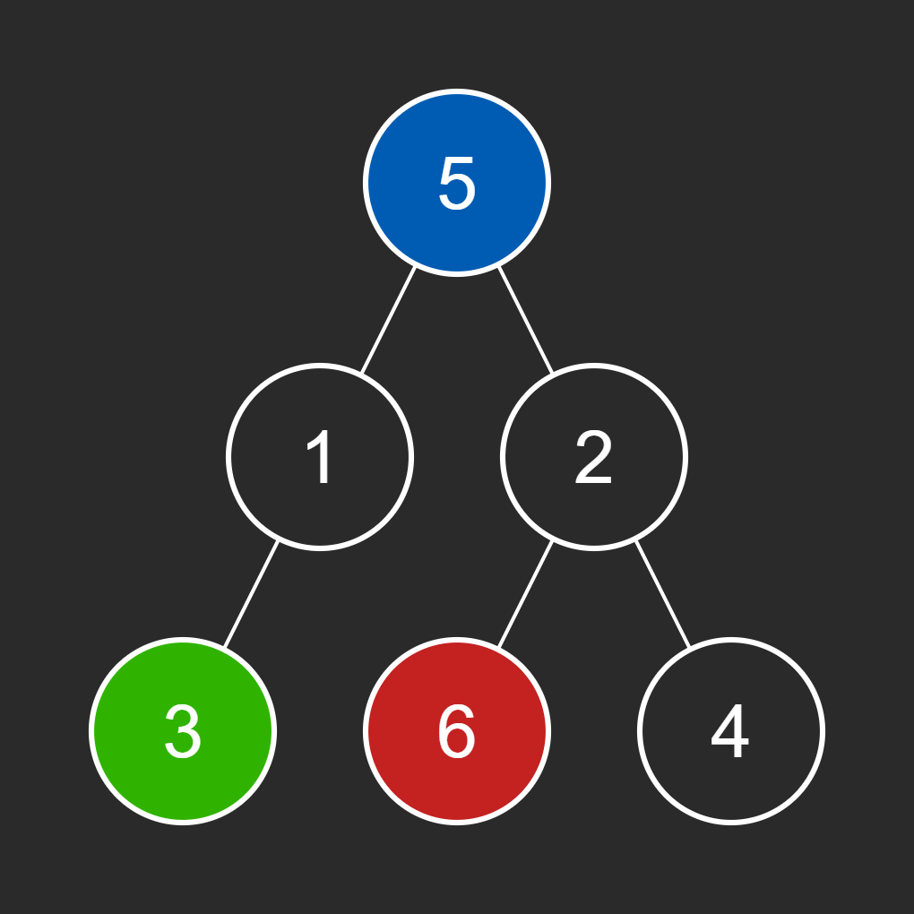
The LCA is determined to be node 5, as both left and right subtrees return non-None values.
An image of the tree with the LCA (node 5) highlighted is shown below:
Finding Path to Start:
findPathis called withlowest_common_ancestor(node 5) andstart_value(3).Iteration 1 (node 5):
Moves left to node 1.
Iteration 2 (node 1):
Moves left to node 3.
Iteration 3 (node 3):
Matches
start_value, path is complete.
Final
path_to_start:['L', 'L']
Finding Path to Destination:
findPathis called withlowest_common_ancestor(node 5) anddest_value(6).Iteration 1 (node 5):
Tries left subtree (node 1), backtracks.
Moves right to node 2.
Iteration 2 (node 2):
Moves left to node 6.
Iteration 3 (node 6):
Matches
dest_value, path is complete.
Final
path_to_dest:['R', 'L']
Constructing Final Path:
initial_path:'U' * len(path_to_start)='UU'final_path:''.join(path_to_dest)='RL'result:initial_path + final_path='UURL'
Visual Aid - Path Construction Summary:
Component
Value
Length
Initial Path (U's)
UU2
Final Path
RL2
Result
UURL4
Result Calculation:
The final result
'UURL'represents:'UU': Move up twice from the start node (3) to reach the LCA (5).'R': Move right from the LCA to node 2.'L': Move left from node 2 to reach the destination node (6).
The function returns 'UURL' as the shortest path from node 3 to node 6 in the given binary tree.
Approach 2: Path Comparison with Common Prefix
Understanding the Core Idea
The central concept of this solution is to leverage full path construction from the root to both the start and destination nodes, followed by a comparison to identify the point of divergence. This approach effectively breaks down the problem into three main steps: finding complete paths, identifying the common prefix, and constructing the final path.
Full Path Construction: The solution begins by finding the complete paths from the root to both the start node and the destination node. This is done using a depth-first search (DFS) approach.
Common Prefix Identification: Once both paths are constructed, the algorithm identifies the longest common prefix between these paths. This common prefix represents the shared path from the root to the lowest common ancestor (LCA) of the start and destination nodes.
Path Combination: The final step involves constructing the result by combining:
A series of 'U' moves to go up from the start node to the LCA.
The remaining path from the LCA to the destination node.
Code Walkthrough
Defining the Helper Function:
def findPath(current_node: BinaryTreeNode, target_value: int, path: List[str]) -> bool: # ... (function body)This helper function is defined within the main function to encapsulate the task of finding a path from a given node to a target node. It's a crucial part of the solution as it will be used to find paths from the root to both the start and destination nodes.
Path Finding Implementation:
def findPath(current_node: BinaryTreeNode, target_value: int, path: List[str]) -> bool: # Recursively find the path to target node, # appending directions to 'path' if current_node.val == target_value: return True if current_node.left: path.append('L') if findPath(current_node.left, target_value, path): return True path.pop() if current_node.right: path.append('R') if findPath(current_node.right, target_value, path): return True path.pop() return FalseThis function uses a depth-first search approach to find the path from the current node to the target node. It appends 'L' or 'R' to the
pathlist as it traverses left or right. If the target is found, it returnsTrue, propagating the success upwards. If a path doesn't lead to the target, it backtracks by removing the last direction (path.pop()). This method ensures that only the correct path remains in thepathlist when the function completes successfully.Finding Paths from Root:
# Find paths from root to start and destination nodes path_to_start = [] path_to_dest = [] findPath(root, start_value, path_to_start) findPath(root, dest_value, path_to_dest)Here, we use the
findPathfunction to construct two complete paths: one from the root to the start node and another from the root to the destination node. This approach differs from the previous solution as it finds full paths from the root instead of paths from the Lowest Common Ancestor (LCA).Identifying the Common Prefix:
# Find the length of the common prefix in both paths common_prefix_length = 0 while (common_prefix_length < len(path_to_start) and common_prefix_length < len(path_to_dest) and path_to_start[common_prefix_length] == path_to_dest[common_prefix_length]): common_prefix_length += 1This step identifies the length of the common prefix between the two paths. The common prefix represents the shared path from the root to the LCA of the start and destination nodes. By comparing the paths element by element, we can determine where they diverge, which implicitly identifies the LCA without a separate LCA finding algorithm.
Constructing the Final Path:
# Construct the final path: 'U's to go up to LCA, initial_path = 'U' * (len(path_to_start) - common_prefix_length) # then path down to destination final_path = ''.join(path_to_dest[common_prefix_length:]) return initial_path + final_pathThe final path is constructed in two parts:
initial_path: A string of 'U's with length equal to the number of steps from the start node to the LCA. This is calculated by subtracting the length of the common prefix from the length of the path to the start node.final_path: The path from LCA to the destination node, obtained by slicing thepath_to_destlist from the index where the common prefix ends.
These two parts are concatenated to form the complete path from start to destination via the LCA. This method efficiently constructs the required path without explicitly finding the LCA node.
Complexity Analysis
Time Complexity:
, where is the number of nodes in the binary tree. The time complexity is linear because in the worst case, we need to traverse the entire tree twice - once to find the path to the start node and once for the destination node. The later comparison of paths and construction of the final result are linear in the height of the tree, which is at most in a skewed tree.
Space Complexity:
, where is the height of the binary tree. The space complexity is determined by two factors: The maximum depth of the recursion stack during the DFS traversals, which is at most the height of the tree.
The storage of the two paths (
path_to_startandpath_to_dest), which are also bounded by the height of the tree. In the worst case of a skewed tree, this could be, but for a balanced tree, it would be .
Example
Input:
A visual representation of the binary tree with the green node representing the start node (3) and the red node representing the destination node (6) is shown below:

Step-by-Step Walkthrough:
Initialization:
The function is called with
root(a binary tree with the structure shown in the input),start_value = 3, anddest_value = 6.Two empty lists are initialized:
path_to_start = []andpath_to_dest = [].
Finding Path to Start:
The
findPathfunction is called with the root node (value 5) andstart_value(3).Iteration 1 (node 5):
Moves left to node 1.
Iteration 2 (node 1):
Moves left to node 3.
Iteration 3 (node 3):
Matches
start_value, path is complete.
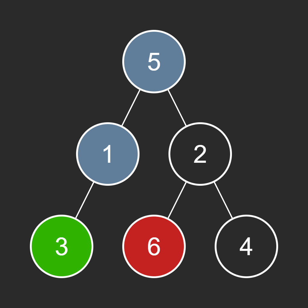
Final
path_to_start:['L', 'L']An image of the path from the root to the start node (3) is shown below:
Finding Path to Destination:
The
findPathfunction is called with the root node (value 5) anddest_value(6).Iteration 1 (node 5):
Tries left subtree (node 1), backtracks.
Moves right to node 2.
Iteration 2 (node 2):
Moves left to node 6.
Iteration 3 (node 6):
Matches
dest_value, path is complete.
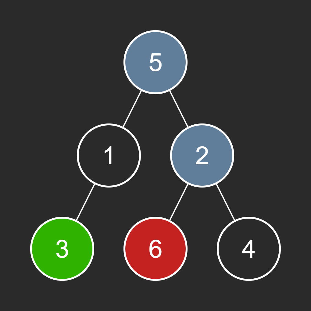
Final
path_to_dest:['R', 'L']An image of the path from the root to the destination node (6) is shown below:
Finding Common Prefix:
The algorithm compares
path_to_startandpath_to_destto find the common prefix.In this case, there is no common prefix as the paths diverge from the root.
Common Prefix Length: 0
Constructing Final Path:
initial_path:'U' * (len(path_to_start) - common_prefix_length)='UU'final_path:''.join(path_to_dest[common_prefix_length:])='RL'result:initial_path + final_path='UURL'
Visual Aid - Path Construction Summary:
Component
Value
Length
Path to Start
LL2
Path to Destination
RL2
Common Prefix
0
Initial Path (U's)
UU2
Final Path
RL2
Result
UURL4
Result Calculation:
The final result
'UURL'represents:'UU': Move up twice from the start node (3) to reach the root (5).'R': Move right from the root to node 2.'L': Move left from node 2 to reach the destination node (6).
The function returns 'UURL' as the shortest path from node 3 to node 6 in the given binary tree.
July 17 -> 1110. Delete Nodes And Return Forest
Given the root of a binary tree, each node in the tree has a distinct value.
After deleting all nodes with a value in to_delete, we are left with a forest (a disjoint union of trees).
Return the roots of the trees in the remaining forest. You may return the result in any order.
Example 1:
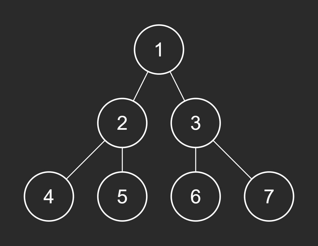
Input: root = [1,2,3,4,5,6,7], to_delete = [3,5]
Output: [[1,2,null,4],[6],[7]]
Example 2:
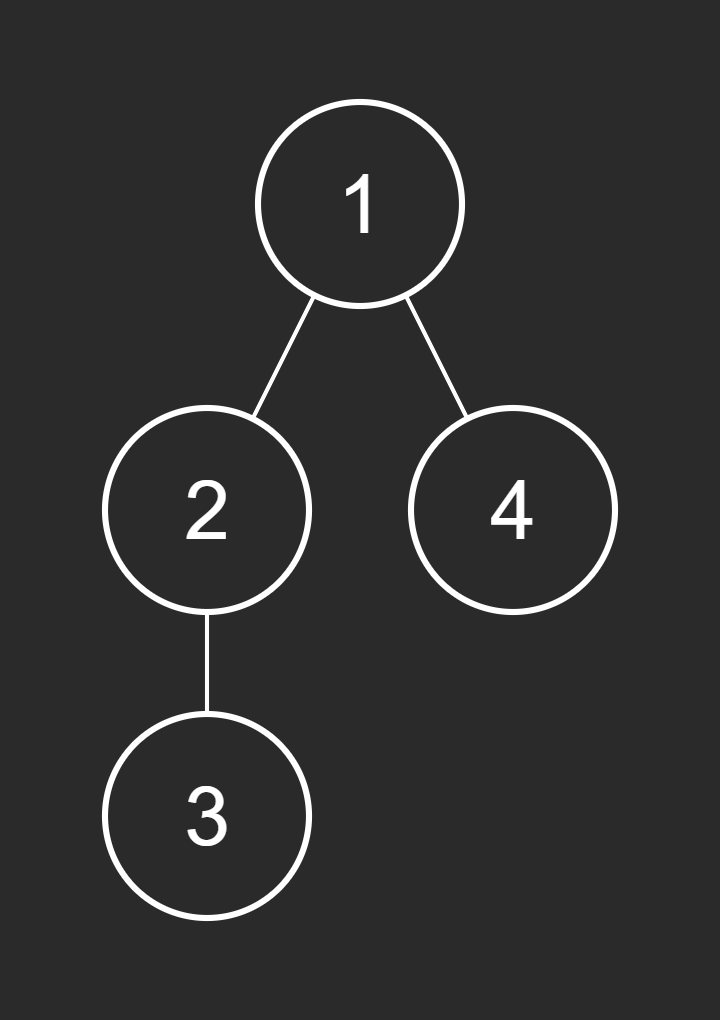
Input: root = [1,2,4,null,3], to_delete = [3]
Output: [[1,2,4]]
Constraints:
The number of nodes in the given tree is at most
1000.Each node has a distinct value between
1and1000.to_delete.length <= 1000to_deletecontains distinct values between1and1000.
Approach 1: Depth-First Traversal with Set-based Deletion
Understanding the Core Idea
The central concept of this solution is to leverage a depth-first traversal (DFS) combined with a set data structure to efficiently delete nodes and construct a forest from a binary tree. This approach allows for a single pass through the tree while simultaneously building the resulting forest.
Depth-First Traversal: The solution uses a post-order traversal to process the tree from bottom to top, ensuring that child nodes are handled before their parents.
Set-based Deletion: By converting the
to_deletelist into a set, the solution achieveslookup time for checking if a node should be deleted. Forest Construction: As nodes are processed, the algorithm builds the forest by adding roots of subtrees that become disconnected due to node deletions.
In-place Modification: The original tree structure is modified in-place, with deleted nodes being replaced by None of their parent's references.
Code Walkthrough
Initialization:
if not root: return [] forest_roots = [] nodes_to_delete = set(to_delete)The function starts by handling the edge case of an empty tree, returning an empty list. It then initializes an empty list
forest_rootsto store the roots of the resulting forest, and converts theto_deletelist into a set forlookup time. Helper Function Definition:
def processNodesAndBuildForest(current_node: BinaryTreeNode) -> ( Optional)[BinaryTreeNode]:A helper function is defined to encapsulate the main logic of processing nodes, deleting specified ones, and building the forest. This function will be called recursively to traverse the tree.
Null Node Handling:
if not current_node: return NoneWithin the helper function, null nodes are immediately returned as None. This serves as the base case for the recursion and handles leaf nodes.
Recursive Processing of Child Nodes:
current_node.left = processNodesAndBuildForest(current_node.left) current_node.right = processNodesAndBuildForest(current_node.right)The function recursively processes the left and right children of the current node. This is a post-order traversal, ensuring that child nodes are processed before their parent. The results of these recursive calls are assigned back to the current node's left and right pointers, potentially modifying the tree structure.
Node Deletion and Forest Building:
if current_node.val in nodes_to_delete: # Add children of deleted node as new roots in the forest if current_node.left: forest_roots.append(current_node.left) if current_node.right: forest_roots.append(current_node.right) return None # Node is deleted by returning None return current_nodeIf the current node's value is in the set of nodes to delete, its children (if they exist) are added to the
forest_rootslist as new roots. The node itself is "deleted" by returning None, which will be assigned to its parent's corresponding child pointer in step 4. If the node is not to be deleted, it's returned as is.Main Tree Processing:
# Process the entire tree root = processNodesAndBuildForest(root)The helper function is called on the root of the tree, starting the traversal and deletion process. The returned value is assigned back to
root, potentially modifying the original tree if the root was deleted.Result Calculation/Return:
# Add the root to `forest_roots` if it wasn't deleted if root: forest_roots.append(root) return forest_rootsAfter processing, if the root still exists (i.e., it wasn't deleted), it's added to the
forest_rootslist. Finally, theforest_rootslist is returned, containing all the roots of the resulting forest.
Complexity Analysis
Time Complexity:
, where is the number of nodes in the binary tree. The algorithm performs a single depth-first traversal of the tree, visiting each node exactly once. The use of a set for to_deleteensures that checking if a node should be deleted is an O(1) operation. Therefore, the overall time complexity is linear with respect to the number of nodes.
Space Complexity:
, where is the height of the tree and is the number of nodes to delete. The recursion stack in the depth-first traversal can go as deep as the height of the tree, contributing
to the space complexity. The
nodes_to_deleteset containselements, contributing to the space complexity. The
forest_rootslist, in the worst case where all nodes are disconnected, could contain up toelements. However, this is bounded by (deleted nodes' children plus potentially the original root), so it doesn't add to the overall complexity. Since in the worst case,
can be equal to (for a skewed tree), and , we can simplify the space complexity to .
Example
Input:
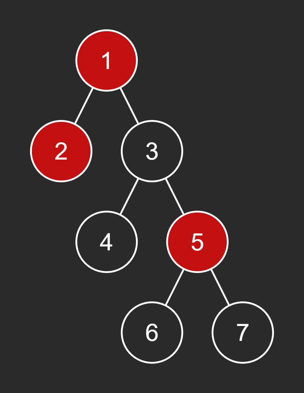
Here's a visual representation of the binary tree with the nodes to delete highlighted in red:
Step-by-Step Walkthrough:
Initialization:
Create an empty list
forest_roots = []to store the roots of the resulting forest.Convert
to_deleteinto a setnodes_to_delete = {1, 2, 5}for efficient lookup.
Main Algorithm Process:
Root Level (Node 1):
Start processing the root node with value 1.
Recursively process the left child (Node 2).
Left Subtree (Node 2):
Process Node 2.
Left and right children are
None, so returnNonefor both.Node 2 is in
nodes_to_delete, so returnNone.Back to Node 1, its left child is now
None.
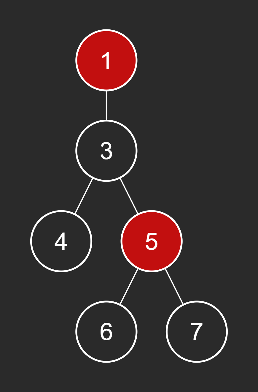
Back to Root Level (Node 1):
Process the right child (Node 3).
Right Subtree (Node 3):
Process Node 3.
Recursively process the left child (Node 4).
Left Subtree of Node 3 (Node 4):
Process Node 4.
Left and right children are
None, so returnNonefor both.Node 4 is not in
nodes_to_delete, so return Node 4.Back to Node 3, its left child remains Node 4.
Back to Node 3:
Process the right child (Node 5).
Right Subtree of Node 3 (Node 5):
Process Node 5.
Recursively process the left child (Node 6).
Left Subtree of Node 5 (Node 6):
Process Node 6.
Left and right children are
None, so returnNonefor both.Node 6 is not in
nodes_to_delete, so return Node 6.Back to Node 5, its left child remains Node 6.
Back to Node 5:
Process the right child (Node 7).
Right Subtree of Node 5 (Node 7):
Process Node 7.
Left and right children are
None, so returnNonefor both.Node 7 is not in
nodes_to_delete, so return Node 7.Back to Node 5, its right child remains Node 7.
Back to Node 5:
Node 5 is in
nodes_to_delete.Add Node 6 and Node 7 to
forest_roots.Return
Noneto Node 3.
Back to Node 3:
Right child is now
None.Node 3 is not in
nodes_to_delete, so return Node 3.
Back to Root Level (Node 1):
Left child is
None, right child is Node 3.Node 1 is in
nodes_to_delete.Add Node 3 to
forest_roots.Return
None.
Final Processing:
The root (Node 1) was deleted, so it's not added to
forest_roots.
Visual Aid: Tree Structure and Deletion Process Here's a summary of the node processing:
Node Value
Action
Children Added to Forest
2
Deleted
None
4
Kept
N/A
6
Kept
N/A
7
Kept
N/A
5
Deleted
6, 7
3
Kept
N/A
1
Deleted
3
Result Calculation:
The
forest_rootslist is built during the traversal.The final
forest_rootscontains [6, 7, 3], representing the roots of the resulting forest.
The algorithm effectively deletes nodes 1, 2, and 5, creating a forest of three trees rooted at nodes 3, 6, and 7. Node 4 remains a child of Node 3 in the resulting structure.
Approach 2: DFS with Root Tracking
Understanding the Core Idea
The central concept of this solution is to leverage a single-pass depth-first search (DFS) with explicit root tracking to efficiently delete nodes and construct a forest from a binary tree. This approach allows for simultaneous node deletion and forest construction in a single traversal.
Single-Pass DFS: The solution uses a pre-order traversal to process the tree from top to bottom, making decisions about node deletion and forest construction as it goes.
Root Tracking: By passing an
is_rootboolean parameter in the recursive calls, the algorithm can determine whether a node should be considered as a potential new root in the forest.Set-based Deletion: Similar to the previous approach, a set is used for
lookup time when checking if a node should be deleted. In-place Modification: The original tree structure is modified in-place, with deleted nodes being replaced by None of their parent's references.
Code Walkthrough
Initialization:
if not root: return [] nodes_to_delete = set(to_delete) forest_roots = []The function begins by handling the edge case of an empty tree, returning an empty list. It then converts the
to_deletelist into a set forlookup time and initializes an empty list forest_rootsto store the roots of the resulting forest.Helper Function Definition:
def processNodesAndBuildForest(current_node: Optional[BinaryTreeNode], is_root: bool) -> Optional[BinaryTreeNode]:A helper function is defined to encapsulate the main logic of processing nodes, handling deletions, and building the forest. This function takes two parameters: the current node and a boolean
is_rootto track potential new roots.Null Node Handling:
if not current_node: return NoneWithin the helper function, null nodes are immediately returned as None. This serves as the base case for the recursion and handles leaf nodes or already deleted subtrees.
Deletion Check:
is_deleted = current_node.val in nodes_to_deleteThe function checks if the current node's value is in the set of nodes to delete, storing the result in
is_deletedfor later use.Root Addition to Forest:
if is_root and not is_deleted: forest_roots.append(current_node)If the current node is a root (either the original root or a child of a deleted node) and it's not meant to be deleted, it's added to the
forest_rootslist. This step is crucial for building the resulting forest.Recursive Processing of Child Nodes:
current_node.left = processNodesAndBuildForest(current_node.left, is_deleted) current_node.right = processNodesAndBuildForest(current_node.right, is_deleted)The function recursively processes the left and right children of the current node. Note that
is_deletedis passed as theis_rootparameter for the child calls. This is because if the current node is deleted, its children become new roots in the forest. The results of these recursive calls are assigned back to the current node's left and right pointers, potentially modifying the tree structure.Node Deletion:
return None if is_deleted else current_nodeIf the current node is to be deleted (
is_deletedis True), the function returns None, effectively removing the node from the tree. Otherwise, it returns the current node unchanged.Main Tree Processing:
processNodesAndBuildForest(root, True)The helper function is called on the root of the tree, with
is_rootset to True, starting the traversal and deletion process.Result Return:
return forest_rootsFinally, the
forest_rootslist is returned, containing all the roots of the resulting forest.
Complexity Analysis
Time Complexity:
, where is the number of nodes in the binary tree. The algorithm performs a single depth-first traversal of the tree, visiting each node exactly once. The use of a set for nodes_to_deleteensures that checking if a node should be deleted is an O(1) operation. Therefore, the overall time complexity is linear with respect to the number of nodes.
Space Complexity:
, where is the height of the tree and is the number of nodes to delete. The recursion stack in the depth-first traversal can go as deep as the height of the tree, contributing
to the space complexity. The
nodes_to_deleteset containselements, contributing to the space complexity. The
forest_rootslist, in the worst case where all nodes are disconnected, could contain up toelements. However, this is bounded by (deleted nodes' children plus potentially the original root), so it doesn't add to the overall complexity. Since in the worst case,
can be equal to (for a skewed tree), and , we can simplify the space complexity to .
Example
Input:
Here's a visual representation of the binary tree with the nodes to delete highlighted in red:

Step-by-Step Walkthrough:
Initialization:
Create a set
nodes_to_delete = {1, 2, 5}for efficient lookup.Initialize an empty list
forest_roots = []to store the roots of the resulting forest.
Main Algorithm Process:
Root Level (Node 1):
Current node: 1, is_root: True
1 is in
nodes_to_delete, so it will be deletedProcess left child (Node 2) with is_root = True
Left Subtree (Node 2):
Current node: 2, is_root: True
2 is in
nodes_to_delete, so it will be deletedProcess left child (None) with is_root = True
Process right child (None) with is_root = True
Return None (Node 2 is deleted)
Back to Root Level (Node 1):
Left child is now None
Process right child (Node 3) with is_root = True
Right Subtree (Node 3):
Current node: 3, is_root: True
3 is not in
nodes_to_delete, so add it toforest_rootsProcess left child (Node 4) with is_root = False
Left Subtree of Node 3 (Node 4):
Current node: 4, is_root: False
4 is not in
nodes_to_deleteProcess left child (None) with is_root = False
Process right child (None) with is_root = False
Return Node 4 (not deleted)
Back to Node 3:
Left child remains Node 4
Process right child (Node 5) with is_root = False
Right Subtree of Node 3 (Node 5):
Current node: 5, is_root: False
5 is in
nodes_to_delete, so it will be deletedProcess left child (Node 6) with is_root = True
Left Subtree of Node 5 (Node 6):
Current node: 6, is_root: True
6 is not in
nodes_to_delete, so add it toforest_rootsProcess left child (None) with is_root = False
Process right child (None) with is_root = False
Return Node 6 (not deleted)
Back to Node 5:
Left child remains Node 6
Process right child (Node 7) with is_root = True
Right Subtree of Node 5 (Node 7):
Current node: 7, is_root: True
7 is not in
nodes_to_delete, so add it toforest_rootsProcess left child (None) with is_root = False
Process right child (None) with is_root = False
Return Node 7 (not deleted)
Back to Node 5:
Right child remains Node 7
Return None (Node 5 is deleted)
Back to Node 3:
Right child is now None
Return Node 3 (not deleted)
Back to Root Level (Node 1):
Right child remains Node 3
Return None (Node 1 is deleted)
Visual Aid: Tree Structure and Deletion Process Here's a summary of the node processing:
Node Value
Action
Was Root
Children
2
Deleted
True
Left: None, Right: None
4
Kept
False
Left: None, Right: None
6
Kept
True
Left: None, Right: None
7
Kept
True
Left: None, Right: None
5
Deleted
False
Left: 6, Right: 7
3
Kept
True
Left: 4, Right: None
1
Deleted
True
Left: None, Right: 3
Result Calculation:
The
forest_rootslist contains [3, 6, 7], representing the roots of the three trees in the resulting forest.
Final Output:
July 18 -> 4. Problem Name
[Problem Statement]
Approach 1: Approach Name
Understanding the Core Idea
...
Code Walkthrough
...
Complexity Analysis
...
Example
...
Approach 2: Approach Name
Understanding the Core Idea
...
Code Walkthrough
...
Complexity Analysis
...
Example
...
July 19 -> 5. Problem Name
[Problem Statement]
Approach 1: Approach Name
Understanding the Core Idea
...
Code Walkthrough
...
Complexity Analysis
...
Example
...
Approach 2: Approach Name
Understanding the Core Idea
...
Code Walkthrough
...
Complexity Analysis
...
Example
...
July 20 -> 6. Problem Name
[Problem Statement]
Approach 1: Approach Name
Understanding the Core Idea
...
Code Walkthrough
...
Complexity Analysis
...
Example
...
Approach 2: Approach Name
Understanding the Core Idea
...
Code Walkthrough
...
Complexity Analysis
...
Example
...
July 21 -> 7. Problem Name
[Problem Statement]
Approach 1: Approach Name
Understanding the Core Idea
...
Code Walkthrough
...
Complexity Analysis
...
Example
...
Approach 2: Approach Name
Understanding the Core Idea
...
Code Walkthrough
...
Complexity Analysis
...
Example
...